import matplotlib.pyplot as plt
import numpy as np
import sympy as sy
import pandas as pd
from scipy.optimize import minimize

Introduction to Linear Regression and Linear Programming

OBJECTIVES

• Derive ordinary least squares models for data

• Evaluate regression models using mean squared error

• Examine errors and assumptions in least squares models

• Use scikit-learn to fit regression models to data

• Set up linear programming problems with constraints using scipy.optimize

Calculus Refresher

An important idea is that of finding a maximum or minimum of a function. From calculus, we have the tools required. Specifically, a maximum or minimum value of a function \(f\) occurs wherever \(f'(x) = 0\) or is underfined. Consider the function:

\[f(x) = x^2\]

def f(x): return x**2
x = np.linspace(-2, 2, 100)
plt.plot(x, f(x))
plt.grid()
plt.title(r'$f(x) = x^2$');

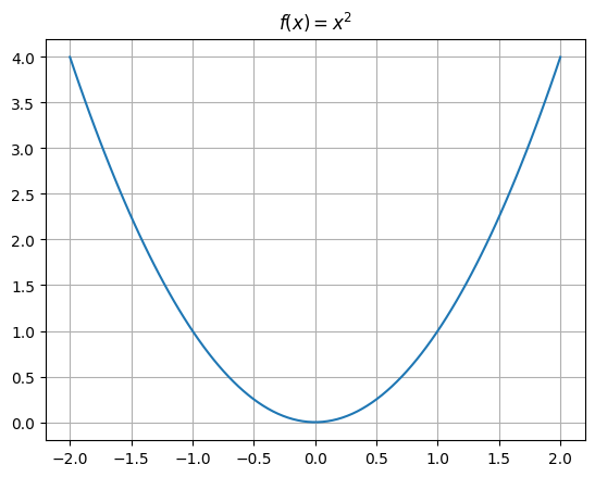
Here, using our power rule for derivatives of polynomials we have:

\[f'(x) = 2x\]

and are left to solve:

\[0 = 2x\]

or

\[x = 0\]

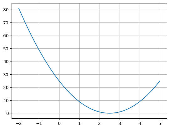
PROBLEM: Use minimize to determine where the function \(f(x) = (5 - 2x)^2\) has a minimum.

def f(x): return (5 - 2*x)**2
x = np.linspace(-2, 5, 100)
plt.plot(x, f(x))
plt.grid();

minimize?

Signature:
minimize(
    fun,
    x0,
    args=(),
    method=None,
    jac=None,
    hess=None,
    hessp=None,
    bounds=None,
    constraints=(),
    tol=None,
    callback=None,
    options=None,
)
Docstring:
Minimization of scalar function of one or more variables.

Parameters
----------
fun : callable
    The objective function to be minimized.

        ``fun(x, *args) -> float``

    where ``x`` is a 1-D array with shape (n,) and ``args``
    is a tuple of the fixed parameters needed to completely
    specify the function.
x0 : ndarray, shape (n,)
    Initial guess. Array of real elements of size (n,),
    where ``n`` is the number of independent variables.
args : tuple, optional
    Extra arguments passed to the objective function and its
    derivatives (`fun`, `jac` and `hess` functions).
method : str or callable, optional
    Type of solver.  Should be one of

        - 'Nelder-Mead' :ref:`(see here) <optimize.minimize-neldermead>`
        - 'Powell'      :ref:`(see here) <optimize.minimize-powell>`
        - 'CG'          :ref:`(see here) <optimize.minimize-cg>`
        - 'BFGS'        :ref:`(see here) <optimize.minimize-bfgs>`
        - 'Newton-CG'   :ref:`(see here) <optimize.minimize-newtoncg>`
        - 'L-BFGS-B'    :ref:`(see here) <optimize.minimize-lbfgsb>`
        - 'TNC'         :ref:`(see here) <optimize.minimize-tnc>`
        - 'COBYLA'      :ref:`(see here) <optimize.minimize-cobyla>`
        - 'SLSQP'       :ref:`(see here) <optimize.minimize-slsqp>`
        - 'trust-constr':ref:`(see here) <optimize.minimize-trustconstr>`
        - 'dogleg'      :ref:`(see here) <optimize.minimize-dogleg>`
        - 'trust-ncg'   :ref:`(see here) <optimize.minimize-trustncg>`
        - 'trust-exact' :ref:`(see here) <optimize.minimize-trustexact>`
        - 'trust-krylov' :ref:`(see here) <optimize.minimize-trustkrylov>`
        - custom - a callable object, see below for description.

    If not given, chosen to be one of ``BFGS``, ``L-BFGS-B``, ``SLSQP``,
    depending on whether or not the problem has constraints or bounds.
jac : {callable,  '2-point', '3-point', 'cs', bool}, optional
    Method for computing the gradient vector. Only for CG, BFGS,
    Newton-CG, L-BFGS-B, TNC, SLSQP, dogleg, trust-ncg, trust-krylov,
    trust-exact and trust-constr.
    If it is a callable, it should be a function that returns the gradient
    vector:

        ``jac(x, *args) -> array_like, shape (n,)``

    where ``x`` is an array with shape (n,) and ``args`` is a tuple with
    the fixed parameters. If `jac` is a Boolean and is True, `fun` is
    assumed to return a tuple ``(f, g)`` containing the objective
    function and the gradient.
    Methods 'Newton-CG', 'trust-ncg', 'dogleg', 'trust-exact', and
    'trust-krylov' require that either a callable be supplied, or that
    `fun` return the objective and gradient.
    If None or False, the gradient will be estimated using 2-point finite
    difference estimation with an absolute step size.
    Alternatively, the keywords  {'2-point', '3-point', 'cs'} can be used
    to select a finite difference scheme for numerical estimation of the
    gradient with a relative step size. These finite difference schemes
    obey any specified `bounds`.
hess : {callable, '2-point', '3-point', 'cs', HessianUpdateStrategy}, optional
    Method for computing the Hessian matrix. Only for Newton-CG, dogleg,
    trust-ncg, trust-krylov, trust-exact and trust-constr.
    If it is callable, it should return the Hessian matrix:

        ``hess(x, *args) -> {LinearOperator, spmatrix, array}, (n, n)``

    where ``x`` is a (n,) ndarray and ``args`` is a tuple with the fixed
    parameters.
    The keywords {'2-point', '3-point', 'cs'} can also be used to select
    a finite difference scheme for numerical estimation of the hessian.
    Alternatively, objects implementing the `HessianUpdateStrategy`
    interface can be used to approximate the Hessian. Available
    quasi-Newton methods implementing this interface are:

        - `BFGS`;
        - `SR1`.

    Not all of the options are available for each of the methods; for
    availability refer to the notes.
hessp : callable, optional
    Hessian of objective function times an arbitrary vector p. Only for
    Newton-CG, trust-ncg, trust-krylov, trust-constr.
    Only one of `hessp` or `hess` needs to be given. If `hess` is
    provided, then `hessp` will be ignored. `hessp` must compute the
    Hessian times an arbitrary vector:

        ``hessp(x, p, *args) ->  ndarray shape (n,)``

    where ``x`` is a (n,) ndarray, ``p`` is an arbitrary vector with
    dimension (n,) and ``args`` is a tuple with the fixed
    parameters.
bounds : sequence or `Bounds`, optional
    Bounds on variables for Nelder-Mead, L-BFGS-B, TNC, SLSQP, Powell,
    trust-constr, and COBYLA methods. There are two ways to specify the
    bounds:

        1. Instance of `Bounds` class.
        2. Sequence of ``(min, max)`` pairs for each element in `x`. None
           is used to specify no bound.

constraints : {Constraint, dict} or List of {Constraint, dict}, optional
    Constraints definition. Only for COBYLA, SLSQP and trust-constr.

    Constraints for 'trust-constr' are defined as a single object or a
    list of objects specifying constraints to the optimization problem.
    Available constraints are:

        - `LinearConstraint`
        - `NonlinearConstraint`

    Constraints for COBYLA, SLSQP are defined as a list of dictionaries.
    Each dictionary with fields:

        type : str
            Constraint type: 'eq' for equality, 'ineq' for inequality.
        fun : callable
            The function defining the constraint.
        jac : callable, optional
            The Jacobian of `fun` (only for SLSQP).
        args : sequence, optional
            Extra arguments to be passed to the function and Jacobian.

    Equality constraint means that the constraint function result is to
    be zero whereas inequality means that it is to be non-negative.
    Note that COBYLA only supports inequality constraints.
tol : float, optional
    Tolerance for termination. When `tol` is specified, the selected
    minimization algorithm sets some relevant solver-specific tolerance(s)
    equal to `tol`. For detailed control, use solver-specific
    options.
options : dict, optional
    A dictionary of solver options. All methods except `TNC` accept the
    following generic options:

        maxiter : int
            Maximum number of iterations to perform. Depending on the
            method each iteration may use several function evaluations.

            For `TNC` use `maxfun` instead of `maxiter`.
        disp : bool
            Set to True to print convergence messages.

    For method-specific options, see :func:`show_options()`.
callback : callable, optional
    A callable called after each iteration.

    All methods except TNC, SLSQP, and COBYLA support a callable with
    the signature:

        ``callback(OptimizeResult: intermediate_result)``

    where ``intermediate_result`` is a keyword parameter containing an
    `OptimizeResult` with attributes ``x`` and ``fun``, the present values
    of the parameter vector and objective function. Note that the name
    of the parameter must be ``intermediate_result`` for the callback
    to be passed an `OptimizeResult`. These methods will also terminate if
    the callback raises ``StopIteration``.

    All methods except trust-constr (also) support a signature like:

        ``callback(xk)``

    where ``xk`` is the current parameter vector.

    Introspection is used to determine which of the signatures above to
    invoke.

Returns
-------
res : OptimizeResult
    The optimization result represented as a ``OptimizeResult`` object.
    Important attributes are: ``x`` the solution array, ``success`` a
    Boolean flag indicating if the optimizer exited successfully and
    ``message`` which describes the cause of the termination. See
    `OptimizeResult` for a description of other attributes.

See also
--------
minimize_scalar : Interface to minimization algorithms for scalar
    univariate functions
show_options : Additional options accepted by the solvers

Notes
-----
This section describes the available solvers that can be selected by the
'method' parameter. The default method is *BFGS*.

**Unconstrained minimization**

Method :ref:`CG <optimize.minimize-cg>` uses a nonlinear conjugate
gradient algorithm by Polak and Ribiere, a variant of the
Fletcher-Reeves method described in [5]_ pp.120-122. Only the
first derivatives are used.

Method :ref:`BFGS <optimize.minimize-bfgs>` uses the quasi-Newton
method of Broyden, Fletcher, Goldfarb, and Shanno (BFGS) [5]_
pp. 136. It uses the first derivatives only. BFGS has proven good
performance even for non-smooth optimizations. This method also
returns an approximation of the Hessian inverse, stored as
`hess_inv` in the OptimizeResult object.

Method :ref:`Newton-CG <optimize.minimize-newtoncg>` uses a
Newton-CG algorithm [5]_ pp. 168 (also known as the truncated
Newton method). It uses a CG method to the compute the search
direction. See also *TNC* method for a box-constrained
minimization with a similar algorithm. Suitable for large-scale
problems.

Method :ref:`dogleg <optimize.minimize-dogleg>` uses the dog-leg
trust-region algorithm [5]_ for unconstrained minimization. This
algorithm requires the gradient and Hessian; furthermore the
Hessian is required to be positive definite.

Method :ref:`trust-ncg <optimize.minimize-trustncg>` uses the
Newton conjugate gradient trust-region algorithm [5]_ for
unconstrained minimization. This algorithm requires the gradient
and either the Hessian or a function that computes the product of
the Hessian with a given vector. Suitable for large-scale problems.

Method :ref:`trust-krylov <optimize.minimize-trustkrylov>` uses
the Newton GLTR trust-region algorithm [14]_, [15]_ for unconstrained
minimization. This algorithm requires the gradient
and either the Hessian or a function that computes the product of
the Hessian with a given vector. Suitable for large-scale problems.
On indefinite problems it requires usually less iterations than the
`trust-ncg` method and is recommended for medium and large-scale problems.

Method :ref:`trust-exact <optimize.minimize-trustexact>`
is a trust-region method for unconstrained minimization in which
quadratic subproblems are solved almost exactly [13]_. This
algorithm requires the gradient and the Hessian (which is
*not* required to be positive definite). It is, in many
situations, the Newton method to converge in fewer iterations
and the most recommended for small and medium-size problems.

**Bound-Constrained minimization**

Method :ref:`Nelder-Mead <optimize.minimize-neldermead>` uses the
Simplex algorithm [1]_, [2]_. This algorithm is robust in many
applications. However, if numerical computation of derivative can be
trusted, other algorithms using the first and/or second derivatives
information might be preferred for their better performance in
general.

Method :ref:`L-BFGS-B <optimize.minimize-lbfgsb>` uses the L-BFGS-B
algorithm [6]_, [7]_ for bound constrained minimization.

Method :ref:`Powell <optimize.minimize-powell>` is a modification
of Powell's method [3]_, [4]_ which is a conjugate direction
method. It performs sequential one-dimensional minimizations along
each vector of the directions set (`direc` field in `options` and
`info`), which is updated at each iteration of the main
minimization loop. The function need not be differentiable, and no
derivatives are taken. If bounds are not provided, then an
unbounded line search will be used. If bounds are provided and
the initial guess is within the bounds, then every function
evaluation throughout the minimization procedure will be within
the bounds. If bounds are provided, the initial guess is outside
the bounds, and `direc` is full rank (default has full rank), then
some function evaluations during the first iteration may be
outside the bounds, but every function evaluation after the first
iteration will be within the bounds. If `direc` is not full rank,
then some parameters may not be optimized and the solution is not
guaranteed to be within the bounds.

Method :ref:`TNC <optimize.minimize-tnc>` uses a truncated Newton
algorithm [5]_, [8]_ to minimize a function with variables subject
to bounds. This algorithm uses gradient information; it is also
called Newton Conjugate-Gradient. It differs from the *Newton-CG*
method described above as it wraps a C implementation and allows
each variable to be given upper and lower bounds.

**Constrained Minimization**

Method :ref:`COBYLA <optimize.minimize-cobyla>` uses the
Constrained Optimization BY Linear Approximation (COBYLA) method
[9]_, [10]_, [11]_. The algorithm is based on linear
approximations to the objective function and each constraint. The
method wraps a FORTRAN implementation of the algorithm. The
constraints functions 'fun' may return either a single number
or an array or list of numbers.

Method :ref:`SLSQP <optimize.minimize-slsqp>` uses Sequential
Least SQuares Programming to minimize a function of several
variables with any combination of bounds, equality and inequality
constraints. The method wraps the SLSQP Optimization subroutine
originally implemented by Dieter Kraft [12]_. Note that the
wrapper handles infinite values in bounds by converting them into
large floating values.

Method :ref:`trust-constr <optimize.minimize-trustconstr>` is a
trust-region algorithm for constrained optimization. It swiches
between two implementations depending on the problem definition.
It is the most versatile constrained minimization algorithm
implemented in SciPy and the most appropriate for large-scale problems.
For equality constrained problems it is an implementation of Byrd-Omojokun
Trust-Region SQP method described in [17]_ and in [5]_, p. 549. When
inequality constraints are imposed as well, it swiches to the trust-region
interior point method described in [16]_. This interior point algorithm,
in turn, solves inequality constraints by introducing slack variables
and solving a sequence of equality-constrained barrier problems
for progressively smaller values of the barrier parameter.
The previously described equality constrained SQP method is
used to solve the subproblems with increasing levels of accuracy
as the iterate gets closer to a solution.

**Finite-Difference Options**

For Method :ref:`trust-constr <optimize.minimize-trustconstr>`
the gradient and the Hessian may be approximated using
three finite-difference schemes: {'2-point', '3-point', 'cs'}.
The scheme 'cs' is, potentially, the most accurate but it
requires the function to correctly handle complex inputs and to
be differentiable in the complex plane. The scheme '3-point' is more
accurate than '2-point' but requires twice as many operations. If the
gradient is estimated via finite-differences the Hessian must be
estimated using one of the quasi-Newton strategies.

**Method specific options for the** `hess` **keyword**

+--------------+------+----------+-------------------------+-----+
| method/Hess  | None | callable | '2-point/'3-point'/'cs' | HUS |
+==============+======+==========+=========================+=====+
| Newton-CG    | x    | (n, n)   | x                       | x   |
|              |      | LO       |                         |     |
+--------------+------+----------+-------------------------+-----+
| dogleg       |      | (n, n)   |                         |     |
+--------------+------+----------+-------------------------+-----+
| trust-ncg    |      | (n, n)   | x                       | x   |
+--------------+------+----------+-------------------------+-----+
| trust-krylov |      | (n, n)   | x                       | x   |
+--------------+------+----------+-------------------------+-----+
| trust-exact  |      | (n, n)   |                         |     |
+--------------+------+----------+-------------------------+-----+
| trust-constr | x    | (n, n)   |  x                      | x   |
|              |      | LO       |                         |     |
|              |      | sp       |                         |     |
+--------------+------+----------+-------------------------+-----+

where LO=LinearOperator, sp=Sparse matrix, HUS=HessianUpdateStrategy

**Custom minimizers**

It may be useful to pass a custom minimization method, for example
when using a frontend to this method such as `scipy.optimize.basinhopping`
or a different library.  You can simply pass a callable as the ``method``
parameter.

The callable is called as ``method(fun, x0, args, **kwargs, **options)``
where ``kwargs`` corresponds to any other parameters passed to `minimize`
(such as `callback`, `hess`, etc.), except the `options` dict, which has
its contents also passed as `method` parameters pair by pair.  Also, if
`jac` has been passed as a bool type, `jac` and `fun` are mangled so that
`fun` returns just the function values and `jac` is converted to a function
returning the Jacobian.  The method shall return an `OptimizeResult`
object.

The provided `method` callable must be able to accept (and possibly ignore)
arbitrary parameters; the set of parameters accepted by `minimize` may
expand in future versions and then these parameters will be passed to
the method.  You can find an example in the scipy.optimize tutorial.

References
----------
.. [1] Nelder, J A, and R Mead. 1965. A Simplex Method for Function
    Minimization. The Computer Journal 7: 308-13.
.. [2] Wright M H. 1996. Direct search methods: Once scorned, now
    respectable, in Numerical Analysis 1995: Proceedings of the 1995
    Dundee Biennial Conference in Numerical Analysis (Eds. D F
    Griffiths and G A Watson). Addison Wesley Longman, Harlow, UK.
    191-208.
.. [3] Powell, M J D. 1964. An efficient method for finding the minimum of
   a function of several variables without calculating derivatives. The
   Computer Journal 7: 155-162.
.. [4] Press W, S A Teukolsky, W T Vetterling and B P Flannery.
   Numerical Recipes (any edition), Cambridge University Press.
.. [5] Nocedal, J, and S J Wright. 2006. Numerical Optimization.
   Springer New York.
.. [6] Byrd, R H and P Lu and J. Nocedal. 1995. A Limited Memory
   Algorithm for Bound Constrained Optimization. SIAM Journal on
   Scientific and Statistical Computing 16 (5): 1190-1208.
.. [7] Zhu, C and R H Byrd and J Nocedal. 1997. L-BFGS-B: Algorithm
   778: L-BFGS-B, FORTRAN routines for large scale bound constrained
   optimization. ACM Transactions on Mathematical Software 23 (4):
   550-560.
.. [8] Nash, S G. Newton-Type Minimization Via the Lanczos Method.
   1984. SIAM Journal of Numerical Analysis 21: 770-778.
.. [9] Powell, M J D. A direct search optimization method that models
   the objective and constraint functions by linear interpolation.
   1994. Advances in Optimization and Numerical Analysis, eds. S. Gomez
   and J-P Hennart, Kluwer Academic (Dordrecht), 51-67.
.. [10] Powell M J D. Direct search algorithms for optimization
   calculations. 1998. Acta Numerica 7: 287-336.
.. [11] Powell M J D. A view of algorithms for optimization without
   derivatives. 2007.Cambridge University Technical Report DAMTP
   2007/NA03
.. [12] Kraft, D. A software package for sequential quadratic
   programming. 1988. Tech. Rep. DFVLR-FB 88-28, DLR German Aerospace
   Center -- Institute for Flight Mechanics, Koln, Germany.
.. [13] Conn, A. R., Gould, N. I., and Toint, P. L.
   Trust region methods. 2000. Siam. pp. 169-200.
.. [14] F. Lenders, C. Kirches, A. Potschka: "trlib: A vector-free
   implementation of the GLTR method for iterative solution of
   the trust region problem", :arxiv:`1611.04718`
.. [15] N. Gould, S. Lucidi, M. Roma, P. Toint: "Solving the
   Trust-Region Subproblem using the Lanczos Method",
   SIAM J. Optim., 9(2), 504--525, (1999).
.. [16] Byrd, Richard H., Mary E. Hribar, and Jorge Nocedal. 1999.
    An interior point algorithm for large-scale nonlinear  programming.
    SIAM Journal on Optimization 9.4: 877-900.
.. [17] Lalee, Marucha, Jorge Nocedal, and Todd Plantega. 1998. On the
    implementation of an algorithm for large-scale equality constrained
    optimization. SIAM Journal on Optimization 8.3: 682-706.

Examples
--------
Let us consider the problem of minimizing the Rosenbrock function. This
function (and its respective derivatives) is implemented in `rosen`
(resp. `rosen_der`, `rosen_hess`) in the `scipy.optimize`.

>>> from scipy.optimize import minimize, rosen, rosen_der

A simple application of the *Nelder-Mead* method is:

>>> x0 = [1.3, 0.7, 0.8, 1.9, 1.2]
>>> res = minimize(rosen, x0, method='Nelder-Mead', tol=1e-6)
>>> res.x
array([ 1.,  1.,  1.,  1.,  1.])

Now using the *BFGS* algorithm, using the first derivative and a few
options:

>>> res = minimize(rosen, x0, method='BFGS', jac=rosen_der,
...                options={'gtol': 1e-6, 'disp': True})
Optimization terminated successfully.
         Current function value: 0.000000
         Iterations: 26
         Function evaluations: 31
         Gradient evaluations: 31
>>> res.x
array([ 1.,  1.,  1.,  1.,  1.])
>>> print(res.message)
Optimization terminated successfully.
>>> res.hess_inv
array([[ 0.00749589,  0.01255155,  0.02396251,  0.04750988,  0.09495377],  # may vary
       [ 0.01255155,  0.02510441,  0.04794055,  0.09502834,  0.18996269],
       [ 0.02396251,  0.04794055,  0.09631614,  0.19092151,  0.38165151],
       [ 0.04750988,  0.09502834,  0.19092151,  0.38341252,  0.7664427 ],
       [ 0.09495377,  0.18996269,  0.38165151,  0.7664427,   1.53713523]])


Next, consider a minimization problem with several constraints (namely
Example 16.4 from [5]_). The objective function is:

>>> fun = lambda x: (x[0] - 1)**2 + (x[1] - 2.5)**2

There are three constraints defined as:

>>> cons = ({'type': 'ineq', 'fun': lambda x:  x[0] - 2 * x[1] + 2},
...         {'type': 'ineq', 'fun': lambda x: -x[0] - 2 * x[1] + 6},
...         {'type': 'ineq', 'fun': lambda x: -x[0] + 2 * x[1] + 2})

And variables must be positive, hence the following bounds:

>>> bnds = ((0, None), (0, None))

The optimization problem is solved using the SLSQP method as:

>>> res = minimize(fun, (2, 0), method='SLSQP', bounds=bnds,
...                constraints=cons)

It should converge to the theoretical solution (1.4 ,1.7).
File:      /Library/Frameworks/Python.framework/Versions/3.12/lib/python3.12/site-packages/scipy/optimize/_minimize.py
Type:      function

x0 = 0
results = minimize(fun = f, x0 = x0)
print(results.x)

[2.49999999]

Using the chain rule

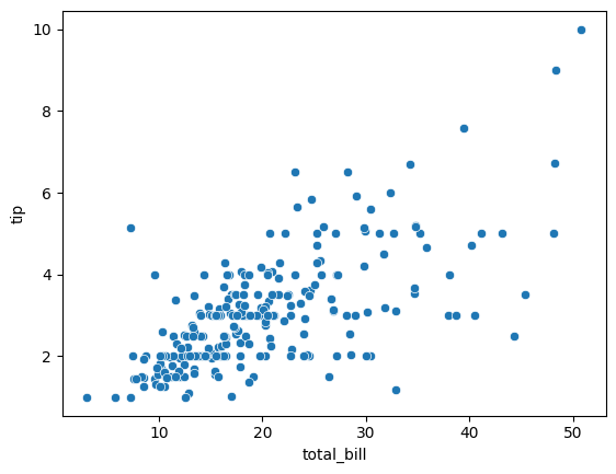
Example 1: Line of best fit

import seaborn as sns

tips = sns.load_dataset('tips')

tips.head()

	total_bill	tip	sex	smoker	day	time	size
0	16.99	1.01	Female	No	Sun	Dinner	2
1	10.34	1.66	Male	No	Sun	Dinner	3
2	21.01	3.50	Male	No	Sun	Dinner	3
3	23.68	3.31	Male	No	Sun	Dinner	2
4	24.59	3.61	Female	No	Sun	Dinner	4

sns.scatterplot(data = tips, x = 'total_bill', y = 'tip');

def y1(x): return .19*x

def y2(x): return .12*x

x = tips['total_bill']

plt.plot(x, y1(x), label = 'y1')
plt.plot(x, y2(x), label = 'y2')
plt.legend()
sns.scatterplot(data = tips, x = 'total_bill', y = 'tip')
plt.title('Which line is a better fit?')
plt.grid();

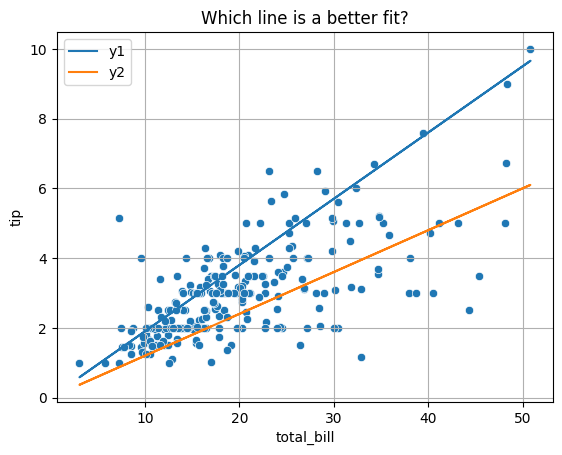
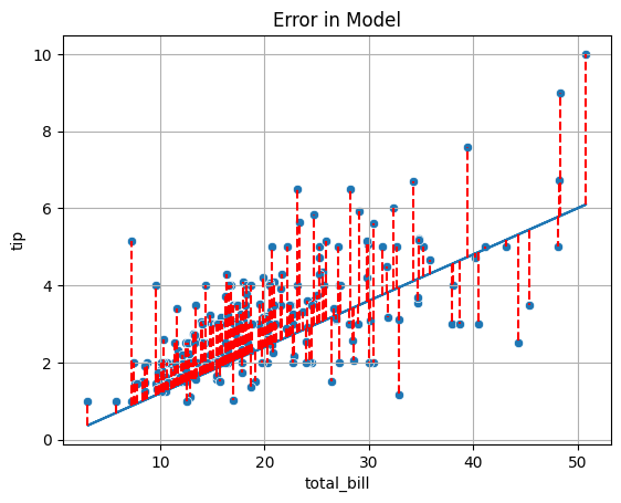
To decide between all possible lines we will examine the error in all these models and select the one that minimizes this error.

plt.plot(x, y2(x))
for i, yhat in enumerate(y2(x)):
    plt.vlines(x = tips['total_bill'].iloc[i], ymin = yhat, ymax = tips['tip'].iloc[i], color = 'red', linestyle = '--')
sns.scatterplot(data = tips, x = 'total_bill', y = 'tip')
plt.title('Error in Model')
plt.grid();

Mean Squared Error

\[\text{MSE}(\beta_0) = \frac{1}{n}\sum_{i = 1}^n (y_i - \beta_0x)^2\]

OBJECTIVE: Minimize mean squared error

def mse(beta):
    return np.mean((y - beta*x)**2)

x = tips['total_bill']
y = tips['tip']

mse(.19)

2.185143996844262

mse(.12)

1.4430533029508197

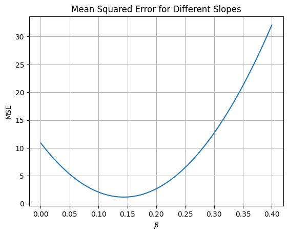
PROBLEM

Use the array of slopes below to loop over each possible slope and determine which gives the lowest Mean Squared Error.

slopes = np.linspace(.1, .2, 11)
slopes

array([0.1 , 0.11, 0.12, 0.13, 0.14, 0.15, 0.16, 0.17, 0.18, 0.19, 0.2 ])

for slope in slopes:
    print(slope, mse(slope))

0.1 2.0777683729508194
0.11 1.7133696722540983
0.12000000000000001 1.4430533029508195
0.13 1.2668192650409837
0.14 1.18466755852459
0.15000000000000002 1.1965981834016395
0.16 1.3026111396721312
0.17 1.502706427336066
0.18 1.7968840463934426
0.19 2.185143996844262
0.2 2.667486278688525

betas = np.linspace(0, .4, 100)
plt.plot(betas, [mse(beta) for beta in betas])
plt.xlabel(r'$\beta$')
plt.ylabel('MSE')
plt.title('Mean Squared Error for Different Slopes')
plt.grid();

Using scipy

To find the minimum of our objective function, the minimize function can again be used. It requires a function to be minimized and an intial guess.

minimize(mse, x0 = .1)

  message: Optimization terminated successfully.
  success: True
   status: 0
      fun: 1.1781161154513358
        x: [ 1.437e-01]
      nit: 1
      jac: [ 1.103e-06]
 hess_inv: [[1]]
     nfev: 6
     njev: 3

Solving the Problem Exactly

From calculus we know that the minimum value for a quadratic will occur where the first derivative equals zero. Thus, to determine the equations for the line of best fit, we minimize the MSE function with respect to \(\beta\).

\[f(\beta) = \frac{1}{n}\sum_{i = 1}^n (y - \beta x)^2\]

\[f'(\beta) = \frac{-2}{n}\sum_{i = 1}^n(y - \beta x) x\]

\[ 0 = \frac{-2}{n}\sum_{i = 1}^n(y - \beta x) x\]

\[0 = \sum_{i = 1}^n(y - \beta x) x\]

\[0 = \sum yx - \sum \beta x^2 \]

\[\sum \beta x^2 = \sum y x\]

\[\beta \sum x^2 = \sum y x\]

\[\beta = \frac{\sum y x}{\sum x^2}\]

np.sum(tips['total_bill']*tips['tip'])/np.sum(tips['total_bill']**2)

0.14373189527721666

Adding an intercept

Consider the model:

\[y = \beta_0 + \beta_1 x + \epsilon\]

where \(\epsilon = N(0, 1)\).

Now, the objective function changes to be a function in 3-Dimensions where the slope and intercept terms are input and mean squared error is the output.

\[\text{MSE}(\beta_0, \beta_1) = \frac{1}{n}\sum_{i = 1}^n (y - (\beta_0 + \beta_1 x)^2)\]

def mse(betas):
    return np.mean((y - (betas[0] + betas[1]*x))**2)

mse([4, 3])

4305.7986356557385

slopes = np.linspace(4, 5, 10)
intercepts = np.linspace(2, 3, 10)
for slope in slopes:
    for intercept in intercepts:
        print(f'Slope {slope: .2f}, Intercept: {intercept: .2f}, MSE: {mse([slope, intercept])}')

Slope  4.00, Intercept:  2.00, MSE: 1930.6791278688527
Slope  4.00, Intercept:  2.11, MSE: 2148.120884836066
Slope  4.00, Intercept:  2.22, MSE: 2377.1777444444447
Slope  4.00, Intercept:  2.33, MSE: 2617.8497066939894
Slope  4.00, Intercept:  2.44, MSE: 2870.1367715846995
Slope  4.00, Intercept:  2.56, MSE: 3134.038939116575
Slope  4.00, Intercept:  2.67, MSE: 3409.556209289617
Slope  4.00, Intercept:  2.78, MSE: 3696.6885821038245
Slope  4.00, Intercept:  2.89, MSE: 3995.436057559198
Slope  4.00, Intercept:  3.00, MSE: 4305.7986356557385
Slope  4.11, Intercept:  2.00, MSE: 1939.7078305606155
Slope  4.11, Intercept:  2.11, MSE: 2157.6381293209874
Slope  4.11, Intercept:  2.22, MSE: 2387.183530722526
Slope  4.11, Intercept:  2.33, MSE: 2628.3440347652295
Slope  4.11, Intercept:  2.44, MSE: 2881.1196414491
Slope  4.11, Intercept:  2.56, MSE: 3145.510350774134
Slope  4.11, Intercept:  2.67, MSE: 3421.516162740336
Slope  4.11, Intercept:  2.78, MSE: 3709.137077347703
Slope  4.11, Intercept:  2.89, MSE: 4008.373094596235
Slope  4.11, Intercept:  3.00, MSE: 4319.224214485935
Slope  4.22, Intercept:  2.00, MSE: 1948.7612246104027
Slope  4.22, Intercept:  2.11, MSE: 2167.180065163935
Slope  4.22, Intercept:  2.22, MSE: 2397.214008358632
Slope  4.22, Intercept:  2.33, MSE: 2638.8630541944963
Slope  4.22, Intercept:  2.44, MSE: 2892.127202671524
Slope  4.22, Intercept:  2.56, MSE: 3157.006453789719
Slope  4.22, Intercept:  2.67, MSE: 3433.500807549079
Slope  4.22, Intercept:  2.78, MSE: 3721.6102639496057
Slope  4.22, Intercept:  2.89, MSE: 4021.334822991298
Slope  4.22, Intercept:  3.00, MSE: 4332.674484674156
Slope  4.33, Intercept:  2.00, MSE: 1957.839310018215
Slope  4.33, Intercept:  2.11, MSE: 2176.746692364906
Slope  4.33, Intercept:  2.22, MSE: 2407.269177352763
Slope  4.33, Intercept:  2.33, MSE: 2649.4067649817853
Slope  4.33, Intercept:  2.44, MSE: 2903.1594552519737
Slope  4.33, Intercept:  2.56, MSE: 3168.527248163327
Slope  4.33, Intercept:  2.67, MSE: 3445.5101437158464
Slope  4.33, Intercept:  2.78, MSE: 3734.1081419095317
Slope  4.33, Intercept:  2.89, MSE: 4034.3212427443837
Slope  4.33, Intercept:  3.00, MSE: 4346.149446220401
Slope  4.44, Intercept:  2.00, MSE: 1966.9420867840518
Slope  4.44, Intercept:  2.11, MSE: 2186.3380109239015
Slope  4.44, Intercept:  2.22, MSE: 2417.349037704918
Slope  4.44, Intercept:  2.33, MSE: 2659.9751671271
Slope  4.44, Intercept:  2.44, MSE: 2914.216399190447
Slope  4.44, Intercept:  2.56, MSE: 3180.07273389496
Slope  4.44, Intercept:  2.67, MSE: 3457.5441712406387
Slope  4.44, Intercept:  2.78, MSE: 3746.630711227484
Slope  4.44, Intercept:  2.89, MSE: 4047.3323538554946
Slope  4.44, Intercept:  3.00, MSE: 4359.649099124672
Slope  4.56, Intercept:  2.00, MSE: 1976.0695549079135
Slope  4.56, Intercept:  2.11, MSE: 2195.9540208409226
Slope  4.56, Intercept:  2.22, MSE: 2427.4535894150986
Slope  4.56, Intercept:  2.33, MSE: 2670.568260630439
Slope  4.56, Intercept:  2.44, MSE: 2925.2980344869466
Slope  4.56, Intercept:  2.56, MSE: 3191.6429109846176
Slope  4.56, Intercept:  2.67, MSE: 3469.6028901234567
Slope  4.56, Intercept:  2.78, MSE: 3759.1779719034603
Slope  4.56, Intercept:  2.89, MSE: 4060.36815632463
Slope  4.56, Intercept:  3.00, MSE: 4373.173443386967
Slope  4.67, Intercept:  2.00, MSE: 1985.2217143897997
Slope  4.67, Intercept:  2.11, MSE: 2205.594722115969
Slope  4.67, Intercept:  2.22, MSE: 2437.5828324833033
Slope  4.67, Intercept:  2.33, MSE: 2681.1860454918037
Slope  4.67, Intercept:  2.44, MSE: 2936.4043611414695
Slope  4.67, Intercept:  2.56, MSE: 3203.2377794323006
Slope  4.67, Intercept:  2.67, MSE: 3481.686300364298
Slope  4.67, Intercept:  2.78, MSE: 3771.7499239374615
Slope  4.67, Intercept:  2.89, MSE: 4073.428650151791
Slope  4.67, Intercept:  3.00, MSE: 4386.722479007286
Slope  4.78, Intercept:  2.00, MSE: 1994.3985652297108
Slope  4.78, Intercept:  2.11, MSE: 2215.2601147490386
Slope  4.78, Intercept:  2.22, MSE: 2447.7367669095324
Slope  4.78, Intercept:  2.33, MSE: 2691.828521711192
Slope  4.78, Intercept:  2.44, MSE: 2947.535379154018
Slope  4.78, Intercept:  2.56, MSE: 3214.8573392380076
Slope  4.78, Intercept:  2.67, MSE: 3493.794401963165
Slope  4.78, Intercept:  2.78, MSE: 3784.3465673294872
Slope  4.78, Intercept:  2.89, MSE: 4086.5138353369757
Slope  4.78, Intercept:  3.00, MSE: 4400.29620598563
Slope  4.89, Intercept:  2.00, MSE: 2003.600107427646
Slope  4.89, Intercept:  2.11, MSE: 2224.950198740134
Slope  4.89, Intercept:  2.22, MSE: 2457.9153926937865
Slope  4.89, Intercept:  2.33, MSE: 2702.495689288606
Slope  4.89, Intercept:  2.44, MSE: 2958.69108852459
Slope  4.89, Intercept:  2.56, MSE: 3226.5015904017396
Slope  4.89, Intercept:  2.67, MSE: 3505.927194920056
Slope  4.89, Intercept:  2.78, MSE: 3796.9679020795384
Slope  4.89, Intercept:  2.89, MSE: 4099.6237118801855
Slope  4.89, Intercept:  3.00, MSE: 4413.894624322
Slope  5.00, Intercept:  2.00, MSE: 2012.8263409836065
Slope  5.00, Intercept:  2.11, MSE: 2234.664974089254
Slope  5.00, Intercept:  2.22, MSE: 2468.1187098360656
Slope  5.00, Intercept:  2.33, MSE: 2713.1875482240443
Slope  5.00, Intercept:  2.44, MSE: 2969.871489253188
Slope  5.00, Intercept:  2.56, MSE: 3238.1705329234965
Slope  5.00, Intercept:  2.67, MSE: 3518.0846792349726
Slope  5.00, Intercept:  2.78, MSE: 3809.6139281876135
Slope  5.00, Intercept:  2.89, MSE: 4112.75827978142
Slope  5.00, Intercept:  3.00, MSE: 4427.517734016393

minimize(mse, [5, 3])

  message: Optimization terminated successfully.
  success: True
   status: 0
      fun: 1.0360194420115216
        x: [ 9.203e-01  1.050e-01]
      nit: 5
      jac: [-5.960e-08 -8.643e-07]
 hess_inv: [[ 2.980e+00 -1.253e-01]
            [-1.253e-01  6.334e-03]]
     nfev: 18
     njev: 6

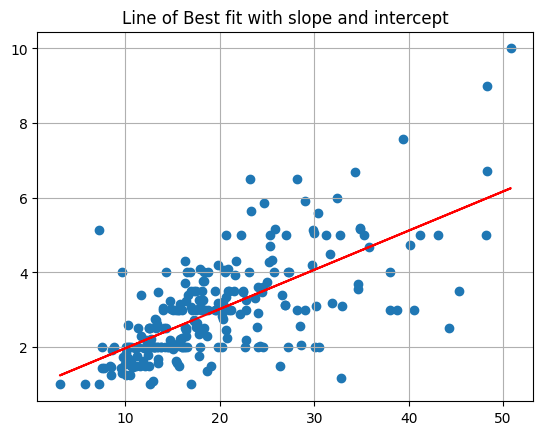
betas = minimize(mse, [0, 0]).x

def lobf(x): return betas[0] + betas[1]*x

plt.scatter(x, y)
plt.plot(x, lobf(x), color = 'red')
plt.grid()
plt.title('Line of Best fit with slope and intercept');

Using scikit-learn

The scikit-learn library has many predictive models and modeling tools. It is a popular library in industry for Machine Learning tasks. docs

# !pip install -U scikit-learn

credit = pd.read_csv('../data/Credit.csv', index_col=0)
credit.head()

	Income	Limit	Rating	Cards	Age	Education	Gender	Student	Married	Ethnicity	Balance
1	14.891	3606	283	2	34	11	Male	No	Yes	Caucasian	333
2	106.025	6645	483	3	82	15	Female	Yes	Yes	Asian	903
3	104.593	7075	514	4	71	11	Male	No	No	Asian	580
4	148.924	9504	681	3	36	11	Female	No	No	Asian	964
5	55.882	4897	357	2	68	16	Male	No	Yes	Caucasian	331

from sklearn.linear_model import LinearRegression

PROBLEM: Which feature is the strongest predictor of Balance in the data?

sns.heatmap(credit.corr(numeric_only = True), annot = True)

<Axes: >

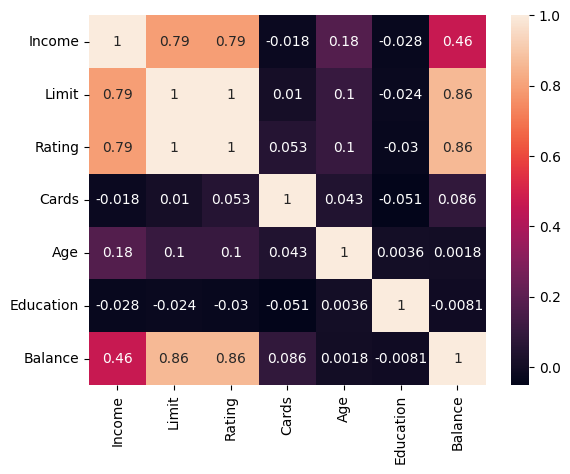
#define X as the feature most correlated with Balance
#and y as Balance
X = credit[['Rating']]
y = credit['Balance']

PROBLEM: Build a LinearRegression model, determine the Root Mean Squared Error and interpret the slope and intercept.

1. Instantiate

2. Fit

3. Predict/score

X.shape, y.shape

((400, 1), (400,))

#instantiate
model = LinearRegression()

#fit
model.fit(X, y)

LinearRegression()

In a Jupyter environment, please rerun this cell to show the HTML representation or trust the notebook.
On GitHub, the HTML representation is unable to render, please try loading this page with nbviewer.org.

#look at coefficient and intercept
model.coef_, model.intercept_

(array([2.56624033]), -390.84634178723786)

yhat = model.predict(X)
yhat[:10]

array([ 335.39967085,  848.64773632,  928.20118647, 1356.76332113,
        525.30145507, 1069.34440447,  273.80990299,  923.06870581,
        291.77358529,  869.17765894])

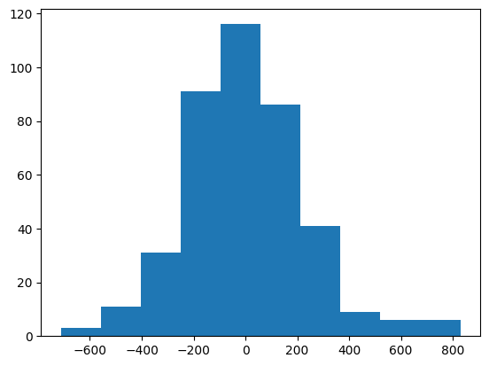
#examine the distribution of errors -- want normal centered at 0
plt.hist((y - yhat))

(array([  3.,  11.,  31.,  91., 116.,  86.,  41.,   9.,   6.,   6.]),
 array([-712.2825064 , -558.1506416 , -404.01877679, -249.88691199,
         -95.75504718,   58.37681762,  212.50868243,  366.64054724,
         520.77241204,  674.90427685,  829.03614165]),
 <BarContainer object of 10 artists>)

model.score(X, y) #r^2 score

0.7458484180585037

from sklearn.metrics import mean_squared_error

#make predictions

#error between true and predicted
mean_squared_error(y, yhat)

53587.80508183237

np.sqrt(mean_squared_error(y, yhat)) #Root Mean Squared Error

231.4903995457098

credit.head(2)

	Income	Limit	Rating	Cards	Age	Education	Gender	Student	Married	Ethnicity	Balance
1	14.891	3606	283	2	34	11	Male	No	Yes	Caucasian	333
2	106.025	6645	483	3	82	15	Female	Yes	Yes	Asian	903

X2 = credit[['Rating', 'Limit', 'Income', 'Age']]

model2 = LinearRegression()
model2.fit(X2, y)

LinearRegression()

In a Jupyter environment, please rerun this cell to show the HTML representation or trust the notebook.
On GitHub, the HTML representation is unable to render, please try loading this page with nbviewer.org.

yhat2 = model2.predict(X2)

np.sqrt(mean_squared_error(y, yhat2))

160.88858783942516

model2.coef_

array([ 2.73142151,  0.08183201, -7.61267561, -0.85611769])

Problem: Determine \(\alpha\) and \(\beta\) of an investment

Consider an investment with return of the market as \(R_M\) (say the S&P) and the return of a stock \(R\) over the same time period.

\[R = \alpha + \beta*R_M + \epsilon\]

import yfinance as yf

data = yf.download(["NVDA", "SPY"], period="5y")
data.head()

data.info()

close = data.iloc[:, [0, 1]]

close.pct_change().plot()

returns = close.pct_change()

sns.regplot(x = returns.iloc[:, 1], y = returns.iloc[:, 0], scatter_kws={'alpha': 0.3})
plt.xlabel('SPY Close Pct Change')
plt.ylabel('NVDA Close Pct Change')
plt.grid();

#instantiate

#fit

#examine our alpha and beta

Problem

Load in the california housing data from the sample_data folder in colab. Use this data to build a regression model with:

1. The most correlated feature to housing prices as input and price as target

2. The five features you believe would be most important

3. Which model has a lower MSE?

Linear Programming: An example

A dog daycare feeds the dogs a diet that requires a minimum of 15 grams of fiber, 30 grams of protein. Each pound of chick peas contains 1 gram of protein, 5 grams of fiber, and 25 grams of fat. Cottage cheese contains 2 grams of protein, 1 gram of fiber, and 14 grams of fat. Suppose that chick peas are priced at 8 USD per pound, and cottage cheese at 6 USD per pound. The nutritionist claims the dogs will not eat more than 285 grams of fat. Your goal is to obtain the most economical solution given these constraints.

This is summarized in the table below:

ingredient	protein	fiber	fat	cost
chick peas	1 g	5 g	25 g	$8
cottage cheese	2 g	1 g	14 g	$6
minimum	15 g	30 g
maximum			285 g

Mathematically, the objective function is:

\[C = 6x + 8y\]

where \(x\) = chick peas and \(y\) = cottage cheese. This is the total cost of the combination of chick peas and cottage cheese.

We will save the coefficients as a list for use later.

c = [6, 8]

Because each pound of chick peas contains 1 gram of protein and each cottage cheese 2 grams, and know this needs to combine to at least 15 grams you have:

\[2x + y \geq 15\]

As for cottage cheese, you have:

\[x + 5y \geq 30\]

As for the fat content, you have:

\[14x + 25y \leq 285\]

Further, the amount of \(x\) and \(y\) must not be negative.

Graphical representation

To visualize the solution, you can imagine each of the constraints as a region. First, functions for these are defined and plotted together.

def cp(x): #chick peas
    return -2*x + 15
def cc(x): #cottage cheese
    return -1/5*x + 30/5
def fat(x): #fat
    return -14/25*x + 285/25
y = 0
x = np.linspace(0, 30, 100)

d = np.linspace(0, 30, 1000)
x, y = np.meshgrid(d, d)
plt.imshow((y > cp(x)) & (y < fat(x)) & (y > cc(x)).astype('int'),
           origin = 'lower',
          cmap = 'Greys',
          extent=(x.min(), x.max(), y.min(), y.max()),
          alpha = 0.4)
plt.plot(d, cc(d), '-', color = 'black', label = 'cottage cheese')

plt.plot(d, cp(d), '-', color = 'blue', label = 'chick peas')

plt.plot(d, fat(d), '-', color = 'red', label = 'fat')
plt.ylim(0, 15)
plt.xlim(0, 20)
plt.title('Feasible region for dog food problem')
plt.grid();

The form of all solutions can be found by rewriting the objective function as:

\[y = -\frac{6}{8}x + \frac{C}{8}\]

Below, different values of \(C\) are plotted against the original region. Note that the objective function will obtain its maximum and minimum values at the vertices of the polygon. Hence, to solve the problem, you need only look to the vertices. These are highlighted in the plot on the right.

# fig, ax = plt.subplots(1, 2, figsize = (30, 10))
for i in range(10, 1000, 10):
    plt.plot(d, -6/8*d + i/8, '--', color = 'black')
plt.plot(d, -6/8*d + i, '--', color = 'black', label = 'slopes of -6/8 + c/8')
d = np.linspace(0, 30, 1000)
x, y = np.meshgrid(d, d)
plt.imshow((y > cp(x)) & (y < fat(x)) & (y > cc(x)).astype('int'),
           origin = 'lower',
          cmap = 'Greys',
          extent=(x.min(), x.max(), y.min(), y.max()),
          alpha = 0.4)
plt.plot(d, cc(d), '-', color = 'black', label = 'cottage cheese')

plt.plot(d, cp(d), '-', color = 'blue', label = 'chick peas')

plt.plot(d, fat(d), '-', color = 'red', label = 'fat')
plt.ylim(0, 15)
plt.xlim(0, 20)
plt.title('Feasible region for dog food problem\nwith possible cost lines')
plt.grid()
plt.legend();

d = np.linspace(0, 30, 1000)
x, y = np.meshgrid(d, d)
plt.imshow((y > cp(x)) & (y < fat(x)) & (y > cc(x)).astype('int'),
           origin = 'lower',
          cmap = 'Greys',
          extent=(x.min(), x.max(), y.min(), y.max()),
          alpha = 0.4)
plt.plot(d, cc(d), '-', color = 'black', label = 'cottage cheese')
plt.plot(15, 3, 'ro', label = 'possible solutions')
plt.plot(d, cp(d), '-', color = 'blue', label = 'chick peas')
plt.plot(d, fat(d), '-', color = 'red', label = 'fat')
plt.ylim(0, 15)
plt.xlim(0, 20)
plt.title('Feasible region for dog food problem')
plt.grid()
plt.plot(5, 5, 'ro')
plt.plot(5/2, 10, 'ro')
plt.legend();

using linprog

To solve the problem using python, scipy.optimize contains the linprog function that will solve this problem. The one exception is that the greater than inequality constraints need to be converted to less thans by multiplying both sides by -1.

\[C = 6x + 8y\]

\[2x + y \geq 15\]

\[x + 5y \geq 30\]

\[14x + 25y \leq 285\]

#cost coeffients
c = [6, 8]
#coefficients of less than problems
A = [[-2, -1], [-1, -5], [14, 25]]
#right side of inequalities
b = [-15, -30, 285]
res = optim.linprog(c, A, b)

res

EXAMPLE

Suppose we have the opportunity to invest in four projects with given cash flows, net present value, and profitability index (\(\frac{NPV}{\text{investment}}\)) given below.

PROJECT	\(C_0\)	\(C_1\)	\(C_2\)	NPV at 10%	Profitability Index
A	-10	-30	5	21	2.1
B	-5	5	2	16	3.2
C	-5	5	15	12	2.4
D	0	-40	60	13	0.4

\[NPV = 21x_A + 16x_B + 12x_C + 13x_D\]

CONSTRAINTS

Cash flows for period 0 must not be greater than 10 million.

\[10x_A + 5x_B + 5x_C + 0x_D \leq 10\]

Total outflow in period 1 must not be greater than 10 million.

\[-30x_A - 5x_B - 5x_C + 40x_D \leq 10\]

Finally the amount of the investment must be positive and we cannot purchase more than one of each.

\[0 \leq x_A \leq 1\]

\[0 \leq x_B \leq 1\]

\[0 \leq x_C \leq 1\]

\[0 \leq x_D \leq 1\]

from scipy.optimize import linprog

coefs = [-21, -16, -12, -13]
constr = [[10, 5, 5, 0],
          [-30, -5, -5, 40]]
right_side = [10, 10]
bounds = [(0, 1), (0, 1), (0, 1), (0, 1)]

linprog(coefs, constr, right_side, bounds = bounds)