Introduction to Classification and K-Nearest Neighbors

Objectives

• Identify Classification problems in supervised learning

• Use KNeighborsClassifier to model classification problems using scikitlearn

• Use StandardScaler to prepare data for KNN models

• Use Pipeline to combine the preprocessing

• Use KNNImputer to impute missing values

import matplotlib.pyplot as plt
import numpy as np
import pandas as pd
import seaborn as sns

from sklearn.model_selection import train_test_split
from sklearn.pipeline import Pipeline
from sklearn.compose import make_column_transformer
from sklearn.neighbors import KNeighborsClassifier
from sklearn.preprocessing import OneHotEncoder, StandardScaler, PolynomialFeatures
from sklearn.datasets import make_blobs

Today you will work together with a neighbor to answer questions based on the code in the notebook. Use the form here to record your work.

A Second Regression Model

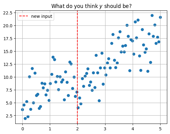
#creating synthetic dataset
x = np.linspace(0, 5, 100)
y = 3*x + 4 + np.random.normal(scale = 3, size = len(x))
df = pd.DataFrame({'x': x, 'y': y})
df.head()

	x	y
0	0.000000	3.669170
1	0.050505	4.575091
2	0.101010	1.898510
3	0.151515	5.199555
4	0.202020	2.297592

#plot data and new observation
plt.scatter(x, y)
plt.axvline(2, color='red', linestyle = '--', label = 'new input')
plt.grid()
plt.legend()
plt.title(r'What do you think $y$ should be?');

KNearest Neighbors

Predict the average of the \(k\) nearest neighbors. One way to think about “nearest” is euclidean distance. We can determine the distance between each data point and the new data point at \(x = 2\) with np.linalg.norm. This is a more general way of determining the euclidean distance between vectors.

#compute distance from each point 
#to new observation
df['distance from x = 2'] = np.linalg.norm(df[['x']] - 2, axis = 1)
df.head()

	x	y	distance from x = 2
0	0.000000	3.669170	2.000000
1	0.050505	4.575091	1.949495
2	0.101010	1.898510	1.898990
3	0.151515	5.199555	1.848485
4	0.202020	2.297592	1.797980

#five nearest points
df.nsmallest(5, 'distance from x = 2')

	x	y	distance from x = 2
40	2.020202	4.009398	0.020202
39	1.969697	7.087389	0.030303
41	2.070707	5.916379	0.070707
38	1.919192	6.202836	0.080808
42	2.121212	4.774703	0.121212

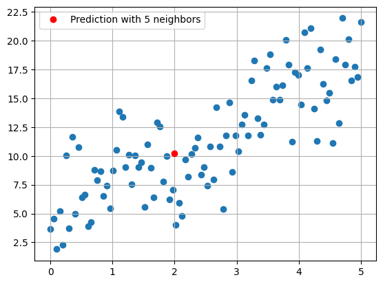
#average of five nearest points
df.nsmallest(5, 'distance from x = 2')['y'].mean()

5.598140955501936

#predicted value with 5 neighbors
plt.scatter(x, y)
plt.plot(2, 10.207196799, 'ro', label = 'Prediction with 5 neighbors')
plt.grid()
plt.legend();

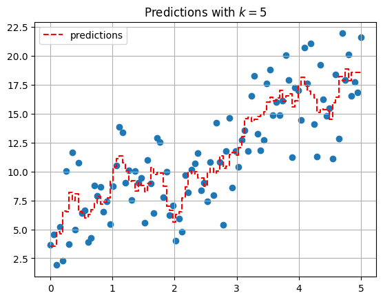
Using sklearn

The KNeighborsRegressor estimator can be used to build the KNN model.

from sklearn.neighbors import KNeighborsRegressor

#predict for all data
knn = KNeighborsRegressor(n_neighbors=5)
knn.fit(x.reshape(-1, 1), y)
predictions = knn.predict(x.reshape(-1, 1))
plt.scatter(x, y)
plt.step(x, predictions, '--r', label = 'predictions')
plt.grid()
plt.legend()
plt.title(r'Predictions with $k = 5$');

from ipywidgets import interact 
import ipywidgets as widgets

def knn_explorer(n_neighbors):
    knn = KNeighborsRegressor(n_neighbors=n_neighbors)
    knn.fit(x.reshape(-1, 1), y)
    predictions = knn.predict(x.reshape(-1, 1))
    plt.scatter(x, y)
    plt.step(x, predictions, '--r', label = 'predictions')
    plt.grid()
    plt.legend()
    plt.title(f'Predictions with $k = {n_neighbors}$');

#explore how predictions change as you change k
interact(knn_explorer, n_neighbors = widgets.IntSlider(value = 1, 
                                                       low = 2, 
                                                       high = len(x)));

Classification

Unlike regression, classification problems involve predicting a categorical variable. For example, the breed of dog, whether or not a customer purchases an item, the presence of a disease, and so on. Today, we will examine the examples of predicting whether or not a person survived the titanic sinking and whether or not a person defaults on their credit card. For each of these problems, we will use the K-Nearest Neighbors algorithm, which we introduce below.

Problem Motivation

#make data
X, y = make_blobs(centers = 2, cluster_std=2, random_state = 42)

#create dataframe
data_1 = pd.DataFrame(X, columns = ['X1', 'X2'])
data_1['y'] = y

#plot sample dataset
sns.scatterplot(data = data_1, x = 'X1', y = 'X2', hue = 'y')
plt.title('Sample Classification Data')
plt.grid();

#dataset with new point
sns.scatterplot(data = data_1, x = 'X1', y = 'X2', hue = 'y')
plt.title('Sample Classification Data')
plt.plot(3, 4, 'ro', markersize = 10, label = 'New Data')
plt.legend()
plt.grid();

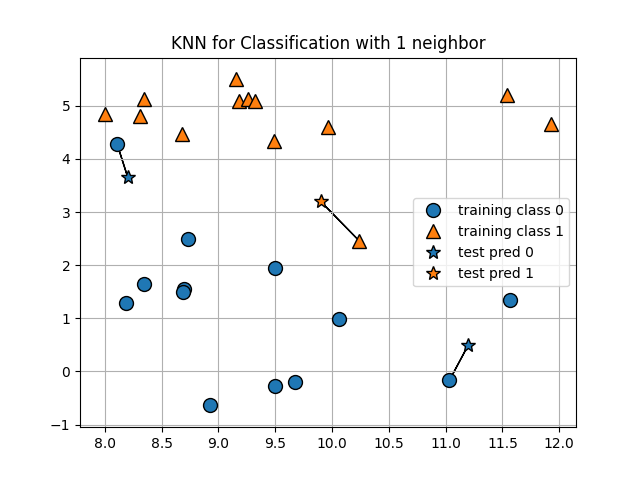
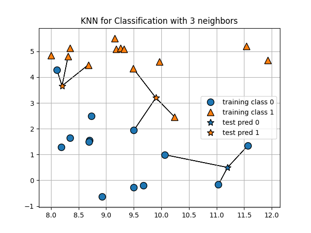
The Intuition

KNN relies on the idea of distance and classifying new datapoints based on the new datapoints distance from known data. There is no equation to be learned as we had with linear regression so we call this a non-parametric model. Essentially, we decide how many points we want to use for voting on the nearness. Below, we demonstrate this with a small sample of the titanic data.

titanic = sns.load_dataset('titanic')

titanic.head()

	survived	pclass	sex	age	sibsp	parch	fare	embarked	class	who	adult_male	deck	embark_town	alive	alone
0	0	3	male	22.0	1	0	7.2500	S	Third	man	True	NaN	Southampton	no	False
1	1	1	female	38.0	1	0	71.2833	C	First	woman	False	C	Cherbourg	yes	False
2	1	3	female	26.0	0	0	7.9250	S	Third	woman	False	NaN	Southampton	yes	True
3	1	1	female	35.0	1	0	53.1000	S	First	woman	False	C	Southampton	yes	False
4	0	3	male	35.0	0	0	8.0500	S	Third	man	True	NaN	Southampton	no	True

#take first five rows as a sample
sample_train = titanic[['pclass', 'age', 'survived']].head()
sample_train

	pclass	age	survived
0	3	22.0	0
1	1	38.0	1
2	3	26.0	1
3	1	35.0	1
4	3	35.0	0

#select a row as a new example to make a prediction on
new_data = titanic[['pclass', 'age']].iloc[30]

new_data

pclass     1.0
age       40.0
Name: 30, dtype: float64

#distance from new data to first example in sample
np.linalg.norm(sample_train.iloc[0, :2] - new_data)

18.110770276274835

#distance between new data and all sample data points
#apply can be used to apply a function to all rows of a DataFrame
distances = sample_train[['pclass', 'age']].apply(lambda x: np.linalg.norm(x - new_data), axis = 1)
distances

0    18.110770
1     2.000000
2    14.142136
3     5.000000
4     5.385165
dtype: float64

#create a column of distances between data and new observation
sample_train['distance'] = distances

sample_train

	pclass	age	survived	distance
0	3	22.0	0	18.110770
1	1	38.0	1	2.000000
2	3	26.0	1	14.142136
3	1	35.0	1	5.000000
4	3	35.0	0	5.385165

#sort by least distance to new data point
sample_train.sort_values('distance')

	pclass	age	survived	distance
1	1	38.0	1	2.000000
3	1	35.0	1	5.000000
4	3	35.0	0	5.385165
2	3	26.0	1	14.142136
0	3	22.0	0	18.110770

Question

If you determine the outcome based on the 1 nearest neighbor, what would you predict? 3 nearest neighbors?

titanic.info()

Using KNeighborsClassifier

The KNeighborsClassifier works just like the earlier LinearRegression estimator. You will instantiate, fit, predict, and score the model as before. Additionally, we have a parameter n_neighbors that will control how many neighbors we make our classification by. To begin, let us form our training and testing data using pclass and age with 5 neighbors.

# X and y
titanic = titanic.dropna()
X = titanic[['pclass', 'age']]
y = titanic['survived']

# train/test split
# random_state = 22
X_train, X_test, y_train, y_test = train_test_split(X, y, random_state=22)

# instantiate
knn = KNeighborsClassifier(n_neighbors=5)

# fit
knn.fit(X_train, y_train)

# score
knn.score(X_train, y_train)

knn.score(X_test, y_test)

.score

Here, we score the model using the total percent correct or accuracy. Later, we will explore additional metrics for classification but for now this is an intuitive way to score a classifier.

\[\text{accuracy} = \frac{\text{number correct}}{\text{number total}}\]

Comparing to Baseline

Typically, you will use the majority class to serve as a baseline predictor. Here, assume you predict just guessing what the majority class is. For this example, it is easy to use the .value_counts(normalize = True) to create a baseline accuracy.

X_train.head()

#baseline
y_train.value_counts(normalize = True)

from sklearn.dummy import DummyClassifier

#which was better?
dummy = DummyClassifier().fit(X_train, y_train)
dummy.score(X_train, y_train)

PROBLEM

Use KNeighborsClassifier to predict the default column using balance and income. Create a train/test split and report the score on both train and test data.

default = pd.read_csv('https://raw.githubusercontent.com/jfkoehler/nyu_bootcamp_fa25/main/data/Default.csv', index_col = 0)
default.head()

	default	student	balance	income
1	No	No	729.526495	44361.625074
2	No	Yes	817.180407	12106.134700
3	No	No	1073.549164	31767.138947
4	No	No	529.250605	35704.493935
5	No	No	785.655883	38463.495879

X = default[['balance', 'income']]
y = default['default']

X_train, X_test, y_train, y_test = train_test_split(X, y, random_state=11)

#baseline on y_train
y_train.value_counts(normalize=True)

default
No     0.965467
Yes    0.034533
Name: proportion, dtype: float64

knn = KNeighborsClassifier()

Improving the Model

Now, we can try two things to improve our model. First, is to change the data we are using and incorporate more features into the model. To do so, we may want to encode categorical features and use these to feed into the model. To do so, we again will use make_column_transformer and select the categorical features to one-hot-encode, while passing the other features through.

default.head(2)

	default	student	balance	income
1	No	No	729.526495	44361.625074
2	No	Yes	817.180407	12106.134700

cat_cols = ['student']
num_cols = ['balance', 'income']
#select columns
X = default.loc[:, cat_cols + num_cols]
y = default['default']

#create OHE
ohe = OneHotEncoder(sparse_output = False, drop = 'if_binary')

#transformer
encoder = make_column_transformer((ohe, cat_cols), 
                                  verbose_feature_names_out=False,
                                  remainder='passthrough')

# train/test
X_train, X_test, y_train, y_test = train_test_split(X, y, random_state=22)

# fit and transform train
X_train_encoded = encoder.fit_transform(X_train)

encoder.get_feature_names_out()

array(['onehotencoder__student_Yes', 'remainder__balance',
       'remainder__income'], dtype=object)

# transform the test
X_test_encoded = encoder.transform(X_test)

# instantiate the KNN estimator
knn = KNeighborsClassifier(n_neighbors=1)

# fit on train
knn.fit(X_train_encoded, y_train)

KNeighborsClassifier(n_neighbors=1)

In a Jupyter environment, please rerun this cell to show the HTML representation or trust the notebook.
On GitHub, the HTML representation is unable to render, please try loading this page with nbviewer.org.

# score on test
knn.score(X_test_encoded, y_test)

0.9556

y_train.value_counts(normalize = True)

default
No     0.966533
Yes    0.033467
Name: proportion, dtype: float64

Another Important Transformation

In addition to using the OneHotEncoder to encode the categorical features, existing numeric features need to be put on the same scale. To do this, we convert the data to \(z\)-scores, computed by:

\[z = \frac{x_i - \mu}{\sigma}\]

You can accomplish this transformation using the StandardScaler. One way to streamline this is to replace the passthrough argument in the make_column_transformer.

# transformer for scaling
encoder = make_column_transformer((ohe, cat_cols), 
                                  remainder=StandardScaler())

# fit and transform
X_train_encoded = encoder.fit_transform(X_train)
# transform
X_test_encoded = encoder.transform(X_test)

# instantiate and fit
knn = KNeighborsClassifier().fit(X_train_encoded, y_train)

# score train and test
print(knn.score(X_train_encoded, y_train))
print(knn.score(X_test_encoded, y_test))

0.976
0.9684

Streamlining data preparation and modeling with Pipeine

The Pipeline object allows you to chain together different transformers and estimator objects from scikitlearn. In our example, this involves first using the make_column_transformer and then to KNearestNeighbor classifier. See the user guide here for more examples.

# create a Pipeline
pipe = Pipeline([('encode', encoder), 
                 ('knn', knn)])

# fit the train data
pipe.fit(X_train, y_train)

/Library/Frameworks/Python.framework/Versions/3.12/lib/python3.12/site-packages/sklearn/compose/_column_transformer.py:1623: FutureWarning: 
The format of the columns of the 'remainder' transformer in ColumnTransformer.transformers_ will change in version 1.7 to match the format of the other transformers.
At the moment the remainder columns are stored as indices (of type int). With the same ColumnTransformer configuration, in the future they will be stored as column names (of type str).
To use the new behavior now and suppress this warning, use ColumnTransformer(force_int_remainder_cols=False).

  warnings.warn(

Pipeline(steps=[('encode',
                 ColumnTransformer(remainder=StandardScaler(),
                                   transformers=[('onehotencoder',
                                                  OneHotEncoder(drop='if_binary',
                                                                sparse_output=False),
                                                  ['student'])])),
                ('knn', KNeighborsClassifier())])

In a Jupyter environment, please rerun this cell to show the HTML representation or trust the notebook.
On GitHub, the HTML representation is unable to render, please try loading this page with nbviewer.org.

# score the train and test
pipe.score(X_train, y_train)

0.976

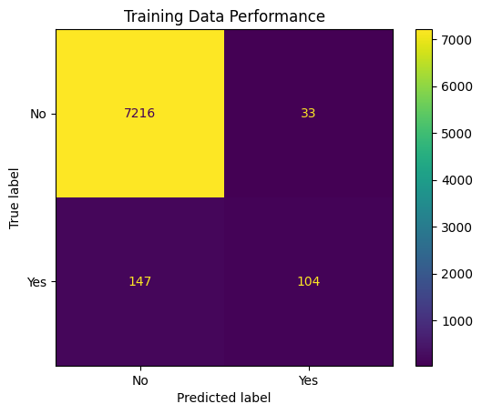
Visualizing Performance

sklearn offers a few visualizers for evaluating a classification model. An important starting one is the ConfusionMatrixDisplay tool, demonstrated below.

from sklearn.metrics import ConfusionMatrixDisplay

cmat = ConfusionMatrixDisplay.from_estimator(pipe, X_train, y_train)
plt.title('Training Data Performance');

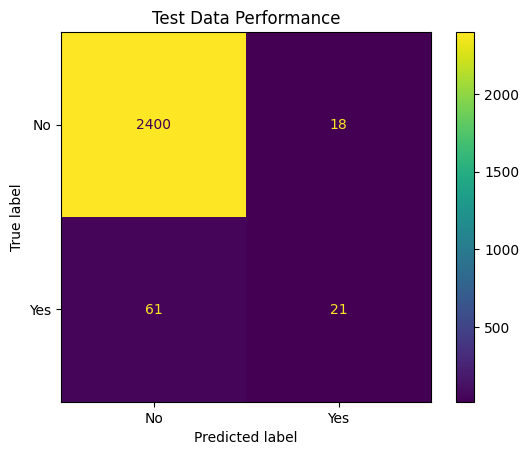
cmat2 = ConfusionMatrixDisplay.from_estimator(pipe, X_test, y_test)
plt.title('Test Data Performance');

Summary

While the KNN model is easy to understand and implement, there are many other classification algorithms that frequently will perform better and contain interpretable parameters. Next class, we will examine one such example with LogisticRegression and the following week we will examine tree models and ensembles.