Reading Files and Split Apply Combine

This lesson focuses on reviewing our basics with pandas and extending them to more advanced munging and cleaning. Specifically, we will discuss how to load data files, work with missing values, use split-apply-combine, use string methods, and work with string and datetime objects. By the end of this lesson you should feel confident doing basic exploratory data analysis using pandas.

OBJECTIVES

• Read local files in as DataFrame objects

• Drop missing values

• Replace missing values

• Impute missing values

• Use .groupby

• Use built in .dt methods

• Convert columns to pd.datetime datatype

• Work with datetime objects in pandas.

Reading Local Files

To read in a local file, we need to pay close attention to our working directory. This means the current location of your work enviornment with respect to your larger computer filesystem. To find your working directory you can use the os library or if your system executes UNIX commands these can be used.

import os
import numpy as np
import pandas as pd
import matplotlib.pyplot as plt
import seaborn as sns

---------------------------------------------------------------------------
ModuleNotFoundError                       Traceback (most recent call last)
Cell In[1], line 5
      3 import pandas as pd
      4 import matplotlib.pyplot as plt
----> 5 import seaborn as sns

ModuleNotFoundError: No module named 'seaborn'

#pip install seaborn

#check working directory
os.getcwd()

'/Users/jacobkoehler/Desktop/fall_24/bootcamp_24'

#list all files in directory
os.listdir()

['continuous_starter.ipynb',
 'intro_to_numpy.ipynb',
 'exarr.npy',
 'subplottin.png',
 'bonus',
 'intro_to_plotting.ipynb',
 'numpy-challenge-3.ipynb',
 'requirements.txt',
 'numpy-challenge-1.ipynb',
 'html_data.ipynb',
 'images',
 'references.bib',
 'intro_probability.ipynb',
 'oop.ipynb',
 'notebooks.ipynb',
 'numpy-challenge-2.ipynb',
 'dates_intro_to_plotting.ipynb',
 'python_fundamentals_one.ipynb',
 'intro_to_pandas.ipynb',
 '_toc.yml',
 'logo.png',
 'homework',
 'data_apis.ipynb',
 '_build',
 '_config.yml',
 'python_fundamentals_two.ipynb',
 '.ipynb_checkpoints',
 'syllabus.ipynb',
 '.git',
 'plotting_seaborn.ipynb',
 'data',
 'hyp_testing.ipynb',
 'pandas_II.ipynb']

#what's in the data folder?
os.listdir('data')

['bus.csv',
 'bud.csv',
 'train.pkl',
 'chicago_crimes.csv',
 'bikeshare_data.csv',
 'doge.jpg',
 'polls.csv',
 'gt_drone_racing.csv',
 'Default.csv',
 'mileage.csv',
 'Ames_Housing_Sales.csv',
 'diamonds.csv',
 'wtgain.csv',
 'elecdemand.csv',
 'us-retail-sales.csv',
 'gapminder_all.csv',
 'GPA.xls',
 'w.npy',
 'v.npy',
 'Heart.csv',
 'DRP.csv',
 'Credit.csv',
 'jobs.csv',
 'insurance.csv',
 'airline-passengers.csv',
 'NOISE.csv',
 'uberx.csv',
 'LasVegasTripAdvisorReviews-Dataset.csv',
 'ufo.csv',
 'state_unemployment.csv',
 'tips_miss.csv',
 'book_sales.csv',
 'health_insurance_charges.csv',
 'PABMI.xls',
 'JOCKO.csv',
 'test.pkl',
 'airline.csv',
 '2017.csv',
 'Sample_Workforce_Data_0720.csv',
 'poll_means.csv',
 'salesdaily.csv',
 'doge.npy',
 'X.npy',
 'y.npy',
 'movie_ratings.tsv',
 'churn_missing.csv',
 'mtcars.csv',
 'office_supplies.csv',
 'train.csv',
 'bikeshare.csv',
 'diabetes.csv',
 'NBA_players_2015.csv',
 'df_predictions.pkl',
 'facefr.csv',
 'spotify.csv',
 'ads.csv',
 'pines.csv',
 'cars.csv',
 'geparts.csv',
 'cell_phone_churn.csv',
 'rollingsales_manhattan.csv',
 'AAPL.csv',
 'heart_cleveland_upload.csv']

#what is the path to ufo.csv?
ufo_path = 'data/ufo.csv'

read_csv

Now, using the path to the ufo.csv file, you can create a DataFrame by passing this filepath to the read_csv function.

#read in ufo data
ufo = pd.read_csv(ufo_path)

# look at first 2 rows
ufo.head(2)

	City	Colors Reported	Shape Reported	State	Time
0	Ithaca	NaN	TRIANGLE	NY	6/1/1930 22:00
1	Willingboro	NaN	OTHER	NJ	6/30/1930 20:00

# high level information
ufo.info()

<class 'pandas.core.frame.DataFrame'>
RangeIndex: 80543 entries, 0 to 80542
Data columns (total 5 columns):
 #   Column           Non-Null Count  Dtype 
---  ------           --------------  ----- 
 0   City             80496 non-null  object
 1   Colors Reported  17034 non-null  object
 2   Shape Reported   72141 non-null  object
 3   State            80543 non-null  object
 4   Time             80543 non-null  object
dtypes: object(5)
memory usage: 3.1+ MB

# numerical summaries
ufo.describe()

	City	Colors Reported	Shape Reported	State	Time
count	80496	17034	72141	80543	80543
unique	13504	31	27	52	68901
top	Seattle	ORANGE	LIGHT	CA	7/4/2014 22:00
freq	646	5216	16332	10743	45

# categorical summaries
ufo.describe(include = 'object')

	City	Colors Reported	Shape Reported	State	Time
count	80496	17034	72141	80543	80543
unique	13504	31	27	52	68901
top	Seattle	ORANGE	LIGHT	CA	7/4/2014 22:00
freq	646	5216	16332	10743	45

# all summaries
ufo.describe(include = 'all')

	City	Colors Reported	Shape Reported	State	Time
count	80496	17034	72141	80543	80543
unique	13504	31	27	52	68901
top	Seattle	ORANGE	LIGHT	CA	7/4/2014 22:00
freq	646	5216	16332	10743	45

# tips = sns.load_dataset('tips')
# tips.head()

# tips.describe(include = 'all')

Reading from url

You can also load datasets from urls where a .csv (or other) file live. Github is one example of this. Note that you want to be sure to use the raw version of the file. For example, a github user dsnair has shared datasets from the book Introduction to Statistical Learning at the link below:

dsnair/ISLR

read in the Auto dataset below.

# get url to raw data
auto_url = 'https://raw.githubusercontent.com/dsnair/ISLR/master/data/csv/Auto.csv'

# pass to read_csv
auto = pd.read_csv(auto_url)

#auto.describe?

# look at the first few rows
auto.head(2)

	mpg	cylinders	displacement	horsepower	weight	acceleration	year	origin	name
0	18.0	8	307.0	130	3504	12.0	70	1	chevrolet chevelle malibu
1	15.0	8	350.0	165	3693	11.5	70	1	buick skylark 320

# high level information
auto.info()

<class 'pandas.core.frame.DataFrame'>
RangeIndex: 392 entries, 0 to 391
Data columns (total 9 columns):
 #   Column        Non-Null Count  Dtype  
---  ------        --------------  -----  
 0   mpg           392 non-null    float64
 1   cylinders     392 non-null    int64  
 2   displacement  392 non-null    float64
 3   horsepower    392 non-null    int64  
 4   weight        392 non-null    int64  
 5   acceleration  392 non-null    float64
 6   year          392 non-null    int64  
 7   origin        392 non-null    int64  
 8   name          392 non-null    object 
dtypes: float64(3), int64(5), object(1)
memory usage: 27.7+ KB

Problems

1. Read in the diamonds.csv file from the data folder, and create a DataFrame named diamonds.

diamonds_path = 'data/diamonds.csv'
diamonds = pd.read_csv(diamonds_path)

2. How many diamonds are greater than .5 carat in the data?

diamonds[diamonds['carat'] > .5].shape[0]

35008

3. What is the highest priced diamond in the data?

diamonds.nlargest(1, 'price')

	carat	cut	color	clarity	depth	table	price	x	y	z
27749	2.29	Premium	I	VS2	60.8	60.0	18823	8.5	8.47	5.16

4. Read the data from the caravan.csv file in located here. Assign this to a variable caravan.

caravan = pd.read_csv('https://raw.githubusercontent.com/dsnair/ISLR/refs/heads/master/data/csv/Caravan.csv')
caravan.head()

	MOSTYPE	MAANTHUI	MGEMOMV	MGEMLEEF	MOSHOOFD	MGODRK	MGODPR	MGODOV	MGODGE	MRELGE	...	APERSONG	AGEZONG	AWAOREG	ABRAND	AZEILPL	APLEZIER	AFIETS	AINBOED	ABYSTAND	Purchase
0	33	1	3	2	8	0	5	1	3	7	...	0	0	0	1	0	0	0	0	0	No
1	37	1	2	2	8	1	4	1	4	6	...	0	0	0	1	0	0	0	0	0	No
2	37	1	2	2	8	0	4	2	4	3	...	0	0	0	1	0	0	0	0	0	No
3	9	1	3	3	3	2	3	2	4	5	...	0	0	0	1	0	0	0	0	0	No
4	40	1	4	2	10	1	4	1	4	7	...	0	0	0	1	0	0	0	0	0	No

5 rows × 86 columns

5. How many Yes’s are in the Purchase column of the caravan data? No’s?

caravan['Purchase'].value_counts()

No     5474
Yes     348
Name: Purchase, dtype: int64

Missing Values

Missing values are a common problem in data, whether this is because they are truly missing or there is confusion between the data encoding and the methods you read the data in using.

# re-examine ufo info
ufo.info()

<class 'pandas.core.frame.DataFrame'>
RangeIndex: 80543 entries, 0 to 80542
Data columns (total 5 columns):
 #   Column           Non-Null Count  Dtype 
---  ------           --------------  ----- 
 0   City             80496 non-null  object
 1   Colors Reported  17034 non-null  object
 2   Shape Reported   72141 non-null  object
 3   State            80543 non-null  object
 4   Time             80543 non-null  object
dtypes: object(5)
memory usage: 3.1+ MB

# one-liner to count missing values
ufo.isna().sum()

City                  47
Colors Reported    63509
Shape Reported      8402
State                  0
Time                   0
dtype: int64

# drop missing values
ufo.dropna()

	City	Colors Reported	Shape Reported	State	Time
12	Belton	RED	SPHERE	SC	6/30/1939 20:00
19	Bering Sea	RED	OTHER	AK	4/30/1943 23:00
36	Portsmouth	RED	FORMATION	VA	7/10/1945 1:30
44	Blairsden	GREEN	SPHERE	CA	6/30/1946 19:00
82	San Jose	BLUE	CHEVRON	CA	7/15/1947 21:00
...	...	...	...	...	...
80524	Olympia	RED	LIGHT	WA	9/4/2014 21:10
80525	Iowa City	BLUE	LIGHT	IA	9/4/2014 21:11
80528	North Royalton	RED	TRIANGLE	OH	9/4/2014 21:30
80536	Wyoming	RED	DISK	PA	9/4/2014 23:00
80541	Orland park	RED	LIGHT	IL	9/5/2014 3:43

15510 rows × 5 columns

# fill missing values
ufo.fillna('dunno')

	City	Colors Reported	Shape Reported	State	Time
0	Ithaca	dunno	TRIANGLE	NY	6/1/1930 22:00
1	Willingboro	dunno	OTHER	NJ	6/30/1930 20:00
2	Holyoke	dunno	OVAL	CO	2/15/1931 14:00
3	Abilene	dunno	DISK	KS	6/1/1931 13:00
4	New York Worlds Fair	dunno	LIGHT	NY	4/18/1933 19:00
...	...	...	...	...	...
80538	Neligh	dunno	CIRCLE	NE	9/4/2014 23:20
80539	Uhrichsville	dunno	LIGHT	OH	9/5/2014 1:14
80540	Tucson	RED BLUE	dunno	AZ	9/5/2014 2:40
80541	Orland park	RED	LIGHT	IL	9/5/2014 3:43
80542	Loughman	dunno	LIGHT	FL	9/5/2014 5:30

80543 rows × 5 columns

# replace missing values with most common value
ufo['Shape Reported'].value_counts()

LIGHT        16332
TRIANGLE      7816
CIRCLE        7725
FIREBALL      6249
OTHER         5506
SPHERE        5231
DISK          5226
OVAL          3721
FORMATION     2405
CIGAR         1983
VARIOUS       1957
FLASH         1329
RECTANGLE     1295
CYLINDER      1252
DIAMOND       1152
CHEVRON        940
EGG            733
TEARDROP       723
CONE           310
CROSS          241
DELTA            7
ROUND            2
CRESCENT         2
DOME             1
PYRAMID          1
FLARE            1
HEXAGON          1
Name: Shape Reported, dtype: int64

ufo['Shape Reported'].fillna('LIGHT')

0        TRIANGLE
1           OTHER
2            OVAL
3            DISK
4           LIGHT
           ...   
80538      CIRCLE
80539       LIGHT
80540       LIGHT
80541       LIGHT
80542       LIGHT
Name: Shape Reported, Length: 80543, dtype: object

# be careful with comparisons!!!
ufo[ufo['Shape Reported'] == np.nan]

	City	Colors Reported	Shape Reported	State	Time

Problem

1. Read in the dataset churn_missing.csv in the data folder, assign to a variable churn below.

churn = pd.read_csv('data/churn_missing.csv')

2. Are there any missing values? What columns are they in and how many are there?

churn.info()

<class 'pandas.core.frame.DataFrame'>
RangeIndex: 3333 entries, 0 to 3332
Data columns (total 20 columns):
 #   Column          Non-Null Count  Dtype  
---  ------          --------------  -----  
 0   state           3333 non-null   object 
 1   account_length  3333 non-null   int64  
 2   area_code       3333 non-null   int64  
 3   intl_plan       3333 non-null   object 
 4   vmail_plan      2933 non-null   object 
 5   vmail_message   2933 non-null   float64
 6   day_mins        3333 non-null   float64
 7   day_calls       3333 non-null   int64  
 8   day_charge      3333 non-null   float64
 9   eve_mins        3333 non-null   float64
 10  eve_calls       3333 non-null   int64  
 11  eve_charge      3333 non-null   float64
 12  night_mins      3333 non-null   float64
 13  night_calls     3333 non-null   int64  
 14  night_charge    3333 non-null   float64
 15  intl_mins       3333 non-null   float64
 16  intl_calls      3333 non-null   int64  
 17  intl_charge     3333 non-null   float64
 18  custserv_calls  3333 non-null   int64  
 19  churn           3333 non-null   bool   
dtypes: bool(1), float64(9), int64(7), object(3)
memory usage: 498.1+ KB

3. What do you think we should do about these? Drop, replace, impute?

churn.vmail_message.describe()#I think we want to keep as much as we can and using the mean to fill things in should be okay

count    2933.000000
mean        8.022503
std        13.657855
min         0.000000
25%         0.000000
50%         0.000000
75%        19.000000
max        51.000000
Name: vmail_message, dtype: float64

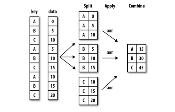
groupby

Often, you are faced with a dataset that you are interested in summaries within groups based on a condition. The simplest condition is that of a unique value in a single column. Using .groupby you can split your data into unique groups and summarize the results.

NOTE: After splitting you need to summarize!

# sample data
df = pd.DataFrame(
    {
        "A": ["foo", "bar", "foo", "bar", "foo", "bar", "foo", "foo"],
        "B": ["one", "one", "two", "three", "two", "two", "one", "three"],
        "C": np.random.randn(8),
        "D": np.random.randn(8),
    }
)
df

	A	B	C	D
0	foo	one	0.014738	-0.549100
1	bar	one	-1.515979	-0.905696
2	foo	two	-1.034411	-0.157872
3	bar	three	0.392896	-1.189066
4	foo	two	-0.260686	-0.671384
5	bar	two	-1.633476	0.943162
6	foo	one	-1.707952	-0.037748
7	foo	three	-0.709300	0.772273

# foo vs. bar
df.groupby('A')['C'].mean()

A
bar   -0.918853
foo   -0.739522
Name: C, dtype: float64

# one two or three?
df.groupby('B').mean(numeric_only=True)

	C	D
B
one	-1.069731	-0.497514
three	-0.158202	-0.208397
two	-0.976191	0.037969

# A and B
df.groupby(['A', 'B']).mean()

		C	D
A	B
bar	one	-1.515979	-0.905696
	three	0.392896	-1.189066
	two	-1.633476	0.943162
foo	one	-0.846607	-0.293424
	three	-0.709300	0.772273
	two	-0.647549	-0.414628

# working with multi-index
df.groupby(['A', 'B'], as_index=False).mean()

	A	B	C	D
0	bar	one	-1.515979	-0.905696
1	bar	three	0.392896	-1.189066
2	bar	two	-1.633476	0.943162
3	foo	one	-0.846607	-0.293424
4	foo	three	-0.709300	0.772273
5	foo	two	-0.647549	-0.414628

# age less than 40 survival rate
titanic = sns.load_dataset('titanic')
titanic.groupby(titanic['age'] < 40)[['survived']].mean()

	survived
age
False	0.332353
True	0.415608

Problems

tips = sns.load_dataset('tips')

tips.head(2)

	total_bill	tip	sex	smoker	day	time	size
0	16.99	1.01	Female	No	Sun	Dinner	2
1	10.34	1.66	Male	No	Sun	Dinner	3

1. Average tip for smokers vs. non-smokers.

tips.groupby('smoker')['tip'].mean()

smoker
Yes    3.008710
No     2.991854
Name: tip, dtype: float64

2. Average bill by day and time.

tips.groupby(['day', 'time'])['total_bill'].mean()

day   time  
Thur  Lunch     17.664754
      Dinner    18.780000
Fri   Lunch     12.845714
      Dinner    19.663333
Sat   Lunch           NaN
      Dinner    20.441379
Sun   Lunch           NaN
      Dinner    21.410000
Name: total_bill, dtype: float64

3. What is another question groupby can help us answer here?

#if size of the party made a difference in tip amount

4. What does the as_index argument do? Demonstrate an example.

#stops the groups from being the index of the result

datetime

A special type of data for pandas are entities that can be considered as dates. We can create a special datatype for these using pd.to_datetime, and access the functions of the datetime module as a result.

# read in the AAPL data
aapl = pd.read_csv('data/AAPL.csv')
aapl.head()

	Date	Open	High	Low	Close	Adj Close	Volume
0	2005-04-25	5.212857	5.288571	5.158571	5.282857	3.522625	186615100
1	2005-04-26	5.254286	5.358572	5.160000	5.170000	3.447372	202626900
2	2005-04-27	5.127143	5.194286	5.072857	5.135714	3.424510	153472200
3	2005-04-28	5.184286	5.191429	5.034286	5.077143	3.385454	143776500
4	2005-04-29	5.164286	5.175714	5.031428	5.151429	3.434988	167907600

# convert to datetime
aapl['Date'] = pd.to_datetime(aapl['Date'])

# extract the month
aapl['month'] = aapl['Date'].dt.month

# extract the day
aapl['day'] = aapl['Date'].dt.day

# set date to be index of data
aapl.set_index('Date', inplace = True)

# sort the index
aapl.sort_index(inplace = True)

# select 2019
aapl.loc['2019']

	Open	High	Low	Close	Adj Close	Volume	month	day
Date
2019-01-02	154.889999	158.850006	154.229996	157.919998	157.245605	37039700	1	2
2019-01-03	143.979996	145.720001	142.000000	142.190002	141.582779	91244100	1	3
2019-01-04	144.529999	148.550003	143.800003	148.259995	147.626846	58607100	1	4
2019-01-07	148.699997	148.830002	145.899994	147.929993	147.298264	54777800	1	7
2019-01-08	149.559998	151.820007	148.520004	150.750000	150.106216	41025300	1	8
...	...	...	...	...	...	...	...	...
2019-04-16	199.460007	201.369995	198.559998	199.250000	199.250000	25696400	4	16
2019-04-17	199.539993	203.380005	198.610001	203.130005	203.130005	28906800	4	17
2019-04-18	203.119995	204.149994	202.520004	203.860001	203.860001	24195800	4	18
2019-04-22	202.830002	204.940002	202.339996	204.529999	204.529999	19439500	4	22
2019-04-23	204.429993	207.750000	203.899994	207.479996	207.479996	23309000	4	23

77 rows × 8 columns

# read back in using parse_dates = True and index_col = 0
aapl = pd.read_csv('data/AAPL.csv', parse_dates=True, index_col=0)
aapl.info()

<class 'pandas.core.frame.DataFrame'>
DatetimeIndex: 3523 entries, 2005-04-25 to 2019-04-23
Data columns (total 6 columns):
 #   Column     Non-Null Count  Dtype  
---  ------     --------------  -----  
 0   Open       3523 non-null   float64
 1   High       3523 non-null   float64
 2   Low        3523 non-null   float64
 3   Close      3523 non-null   float64
 4   Adj Close  3523 non-null   float64
 5   Volume     3523 non-null   int64  
dtypes: float64(5), int64(1)
memory usage: 192.7 KB

from datetime import datetime

# what time is it?
then = datetime.now()
then

datetime.datetime(2023, 10, 4, 21, 45, 49, 915930)

# how much time has passed?
datetime.now() - then

datetime.timedelta(microseconds=6784)

More with timestamps

• Date times: A specific date and time with timezone support. Similar to datetime.datetime from the standard library.

• Time deltas: An absolute time duration. Similar to datetime.timedelta from the standard library.

• Time spans: A span of time defined by a point in time and its associated frequency.

• Date offsets: A relative time duration that respects calendar arithmetic.

# create a pd.Timedelta
pd.Timedelta(5, 'D')

Timedelta('5 days 00:00:00')

# shift a date by 3 months
then + pd.Timedelta(36, 'W')

datetime.datetime(2024, 6, 12, 21, 45, 49, 915930)

Problems

1. Return to the ufo data and convert the Time column to a datetime object.

ufo['Time'] = pd.to_datetime(ufo['Time'])
ufo.info()

<class 'pandas.core.frame.DataFrame'>
RangeIndex: 80543 entries, 0 to 80542
Data columns (total 5 columns):
 #   Column           Non-Null Count  Dtype         
---  ------           --------------  -----         
 0   City             80496 non-null  object        
 1   Colors Reported  17034 non-null  object        
 2   Shape Reported   72141 non-null  object        
 3   State            80543 non-null  object        
 4   Time             80543 non-null  datetime64[ns]
dtypes: datetime64[ns](1), object(4)
memory usage: 3.1+ MB

2. Set the Time column as the index column of the data.

ufo.set_index('Time', inplace = True)

3. Sort it

ufo.sort_index(inplace = True)

4. Create a new dataframe with ufo sightings since January 1, 1999

two_thousands = ufo.loc['1999':]

two_thousands.head()

	City	Colors Reported	Shape Reported	State
Time
1999-01-01 02:30:00	Loma Rica	NaN	LIGHT	CA
1999-01-01 03:00:00	Bauxite	NaN	NaN	AR
1999-01-01 14:00:00	Florence	NaN	CYLINDER	SC
1999-01-01 15:00:00	Lake Henshaw	NaN	CIGAR	CA
1999-01-01 17:15:00	Wilmington Island	NaN	LIGHT	GA