import matplotlib.pyplot as plt
import numpy as np
import sympy as sy
import pandas as pd

---------------------------------------------------------------------------
ModuleNotFoundError                       Traceback (most recent call last)
Cell In[1], line 3
      1 import matplotlib.pyplot as plt
      2 import numpy as np
----> 3 import sympy as sy
      4 import pandas as pd

ModuleNotFoundError: No module named 'sympy'

Introduction to Linear Regression

OBJECTIVES

• Derive ordinary least squares models for data

• Evaluate regression models using mean squared error

• Examine errors and assumptions in least squares models

• Use scikit-learn to fit regression models to data

Calculus Refresher

An important idea is that of finding a maximum or minimum of a function. From calculus, we have the tools required. Specifically, a maximum or minimum value of a function \(f\) occurs wherever \(f'(x) = 0\) or is underfined. Consider the function:

\[f(x) = x^2\]

def f(x): return x**2
x = np.linspace(-2, 2, 100)
plt.plot(x, f(x))
plt.grid()
plt.title(r'$f(x) = x^2$');

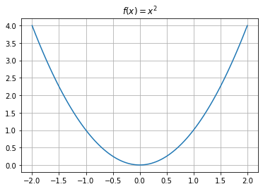
Here, using our power rule for derivatives of polynomials we have:

\[f'(x) = 2x\]

and are left to solve:

\[0 = 2x\]

or

\[x = 0\]

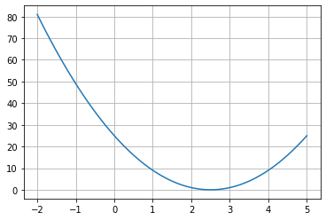
PROBLEM: Determine where the function \(f(x) = (5 - 2x)^2\) has a minimum.

def f(x): return (5 - 2*x)**2
x = np.linspace(-2, 5, 100)
plt.plot(x, f(x))
plt.grid();

Using the chain rule

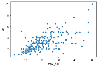
Example 1: Line of best fit

import seaborn as sns

tips = sns.load_dataset('tips')

tips.head()

	total_bill	tip	sex	smoker	day	time	size
0	16.99	1.01	Female	No	Sun	Dinner	2
1	10.34	1.66	Male	No	Sun	Dinner	3
2	21.01	3.50	Male	No	Sun	Dinner	3
3	23.68	3.31	Male	No	Sun	Dinner	2
4	24.59	3.61	Female	No	Sun	Dinner	4

sns.scatterplot(data = tips, x = 'total_bill', y = 'tip');

def y1(x): return .19*x

def y2(x): return .12*x

x = tips['total_bill']

plt.plot(x, y1(x), label = 'y1')
plt.plot(x, y2(x), label = 'y2')
plt.legend()
sns.scatterplot(data = tips, x = 'total_bill', y = 'tip')
plt.title('How to determine the line of best fit?')
plt.grid();

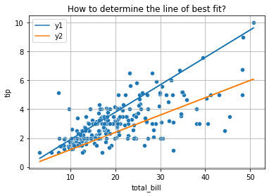
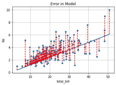
To decide between all possible lines we will examine the error in all these models and select the one that minimizes this error.

plt.plot(x, y2(x))
for i, yhat in enumerate(y2(x)):
    plt.vlines(x = tips['total_bill'].iloc[i], ymin = yhat, ymax = tips['tip'].iloc[i], color = 'red', linestyle = '--')
sns.scatterplot(data = tips, x = 'total_bill', y = 'tip')
plt.title('Error in Model')
plt.grid();

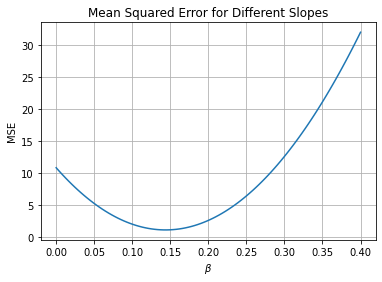
Mean Squared Error

\[\text{MSE}(\beta_0) = \frac{1}{n}\sum_{i = 1}^n (y_i - \beta_0x)^2\]

OBJECTIVE: Minimize mean squared error

def mse(beta):
    return np.mean((y - beta*x)**2)

x = tips['total_bill']
y = tips['tip']

mse(.17)

1.502706427336066

for pct in np.linspace(.1, .2, 11):
    print(f'The MSE for slope {pct: .3f} is {mse(pct): .3f}')

The MSE for slope  0.100 is  2.078
The MSE for slope  0.110 is  1.713
The MSE for slope  0.120 is  1.443
The MSE for slope  0.130 is  1.267
The MSE for slope  0.140 is  1.185
The MSE for slope  0.150 is  1.197
The MSE for slope  0.160 is  1.303
The MSE for slope  0.170 is  1.503
The MSE for slope  0.180 is  1.797
The MSE for slope  0.190 is  2.185
The MSE for slope  0.200 is  2.667

betas = np.linspace(0, .4, 100)
plt.plot(betas, [mse(beta) for beta in betas])
plt.xlabel(r'$\beta$')
plt.ylabel('MSE')
plt.title('Mean Squared Error for Different Slopes')
plt.grid();

Using scipy

To find the minimum of our objective function, the minimize function from scipy.optimize is useful. This relies on a variety of different optimization algorithms to find the minimum of a function.

from scipy.optimize import minimize

minimize(mse, .1 )

  message: Optimization terminated successfully.
  success: True
   status: 0
      fun: 1.1781161154513358
        x: [ 1.437e-01]
      nit: 1
      jac: [ 1.103e-06]
 hess_inv: [[1]]
     nfev: 6
     njev: 3

Solving the Problem Exactly

From calculus we know that the minimum value for a quadratic will occur where the first derivative equals zero. Thus, to determine the equations for the line of best fit, we minimize the MSE function with respect to \(\beta\).

\[f(\beta) = \frac{1}{n}\sum_{i = 1}^n (y - \beta x)^2\]

\[f'(\beta) = \frac{-2}{n}\sum_{i = 1}^n(y - \beta x) x\]

\[ 0 = \frac{-2}{n}\sum_{i = 1}^n(y - \beta x) x\]

\[0 = \sum_{i = 1}^n(y - \beta x) x\]

\[0 = \sum yx - \sum \beta x^2 \]

\[\sum \beta x^2 = \sum y x\]

\[\beta \sum x^2 = \sum y x\]

\[\beta = \frac{\sum y x}{\sum x^2}\]

np.sum(tips['total_bill']*tips['tip'])/np.sum(tips['total_bill']**2)

0.14373189527721666

Adding an intercept

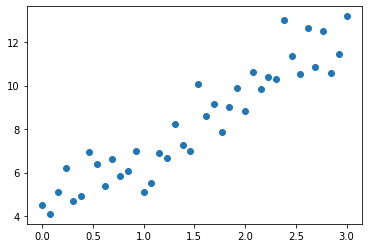
Consider the model:

\[y = \beta_0 + \beta_1 x + \epsilon\]

where \(\epsilon = N(0, 1)\).

np.random.seed(42)
x = np.linspace(0, 3, 40)
y = 3*x + 4 + np.random.normal(size = len(x))
plt.scatter(x, y)

<matplotlib.collections.PathCollection at 0x7f8b45d14250>

Now, the objective function changes to be a function in 3-Dimensions where the slope and intercept terms are input and mean squared error is the output.

\[\text{MSE}(\beta_0, \beta_1) = \frac{1}{n}\sum_{i = 1}^n (y - (\beta_0 + \beta_1 x)^2)\]

def mse(betas):
    return np.mean((y - (betas[0] + betas[1]*x))**2)

mse([4, 3])

0.9329508980248764

minimize(mse, [0, 0])

  message: Optimization terminated successfully.
  success: True
   status: 0
      fun: 0.829630503231984
        x: [ 4.179e+00  2.735e+00]
      nit: 7
      jac: [ 9.686e-08 -2.235e-08]
 hess_inv: [[ 1.921e+00 -9.483e-01]
            [-9.483e-01  6.327e-01]]
     nfev: 24
     njev: 8

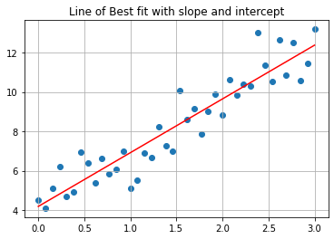
betas = minimize(mse, [0, 0]).x

def lobf(x): return betas[0] + betas[1]*x

plt.scatter(x, y)
plt.plot(x, lobf(x), color = 'red')
plt.grid()
plt.title('Line of Best fit with slope and intercept');

Exercise

Use the minimize function together with your mse function to complete the class below. After calling the fit method assign the slope of the line of best fit to the .coef_ attribute and the \(y\)-intercept to the .intercept_ attribute.

Test your model on the tips data below.

class LinearReg:
    '''
    This class fits an ordinary lease squares model
    of the form beta_0 + beta_1 * x.
    '''
    def __init__(self):
        self.coef_ = None
        self.intercept_ = None
        
    def mse(self, betas):
        return np.mean((y - (betas[0] + betas[1]*x))**2)
        
    def fit(self, x, y):
        #betas that minimize
        betas = minimize(self.mse, [0, 0]).x
        #set coef_
        self.coef_ = betas[1]
        #set intercept_
        self.intercept_ = betas[0]
        
    
    def predict(self, x):
        return self.intercept_ + self.coef_*x
    
    

x = tips['total_bill']
y = tips['tip']

#instantiate the model
model = LinearReg()

#fit the model on data
model.fit(x, y)

#make predictions on all data
model.predict(x)

0      2.704636
1      2.006223
2      3.126835
3      3.407250
4      3.502822
         ...   
239    3.969131
240    3.774836
241    3.301175
242    2.791807
243    2.892630
Name: total_bill, Length: 244, dtype: float64

model.coef_

0.10502447914641161

model.intercept_

0.9202703450693733

A second example

import statsmodels.api as sm
duncan_prestige = sm.datasets.get_rdataset("Duncan", "carData")
print(duncan_prestige.__doc__)

.. container::

   .. container::

      ====== ===============
      Duncan R Documentation
      ====== ===============

      .. rubric:: Duncan's Occupational Prestige Data
         :name: duncans-occupational-prestige-data

      .. rubric:: Description
         :name: description

      The ``Duncan`` data frame has 45 rows and 4 columns. Data on the
      prestige and other characteristics of 45 U. S. occupations in
      1950.

      .. rubric:: Usage
         :name: usage

      .. code:: R

         Duncan

      .. rubric:: Format
         :name: format

      This data frame contains the following columns:

      type
         Type of occupation. A factor with the following levels:
         ``prof``, professional and managerial; ``wc``, white-collar;
         ``bc``, blue-collar.

      income
         Percentage of occupational incumbents in the 1950 US Census who
         earned $3,500 or more per year (about $36,000 in 2017 US
         dollars).

      education
         Percentage of occupational incumbents in 1950 who were high
         school graduates (which, were we cynical, we would say is
         roughly equivalent to a PhD in 2017)

      prestige
         Percentage of respondents in a social survey who rated the
         occupation as “good” or better in prestige

      .. rubric:: Source
         :name: source

      Duncan, O. D. (1961) A socioeconomic index for all occupations. In
      Reiss, A. J., Jr. (Ed.) *Occupations and Social Status.* Free
      Press [Table VI-1].

      .. rubric:: References
         :name: references

      Fox, J. (2016) *Applied Regression Analysis and Generalized Linear
      Models*, Third Edition. Sage.

      Fox, J. and Weisberg, S. (2019) *An R Companion to Applied
      Regression*, Third Edition, Sage.

sns.lmplot(duncan_prestige.data, x = 'education', y = 'prestige')
plt.title('Education vs. Prestige');

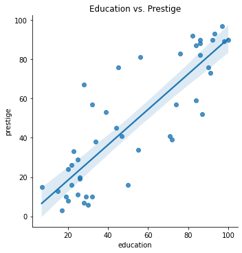
• Fit a model with an intercept to the data.

• What is the slope of the line and what does this mean in terms of education and income?

• What is the intercept of the model and what does this mean in terms of education and income?

x = duncan_prestige.data[['education']]
y = duncan_prestige.data['prestige']

x.shape

(45, 1)

# !pip install -U scikit-learn

from sklearn.linear_model import LinearRegression

model = LinearRegression() #instantiate -- step 1

model.fit(x, y)

LinearRegression()

In a Jupyter environment, please rerun this cell to show the HTML representation or trust the notebook.
On GitHub, the HTML representation is unable to render, please try loading this page with nbviewer.org.

predictions = model.predict(x)
predictions

array([77.85563665, 68.83567885, 83.26761134, 81.46361978, 77.85563665,
       76.05164509, 84.16960712, 90.48357758, 78.75763243, 77.85563665,
       67.03168729, 88.67958602, 87.77759024, 76.05164509, 82.36561556,
       30.95185608, 40.87380966, 50.79576324, 39.97181388, 74.24765353,
       65.22769573, 49.89376746, 64.32569995, 45.38378856, 21.02990249,
       35.46183498, 25.53988139, 29.14786452, 20.12790671, 22.83389405,
       26.44187717,  6.59797001, 23.73588983, 17.42191937, 13.81393625,
       18.32391515, 23.73588983, 25.53988139, 15.61792781, 20.12790671,
       27.34387295, 22.83389405, 18.32391515, 42.67780122, 29.14786452])

model.coef_, model.intercept_

(array([0.90199578]), 0.2839995438216505)

model.coef_[0]

0.9019957803501166

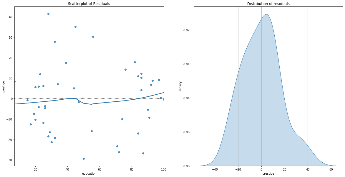
Examining Errors in the Model

Once we have a model, it is important to examine the properties of the residuals. Specifically, we aim to examine the residuals for patterns in error and the overall distribution of these errors.

fig, ax = plt.subplots(1, 2, figsize = (20, 10))
sns.residplot(x = x, y = y, ax = ax[0], lowess=True)
ax[0].set_title('Scatterplot of Residuals')
sns.kdeplot((y - (model.intercept_ + model.coef_[0]*x.values[:, 0])), ax = ax[1], fill = True);
ax[1].grid()
ax[1].set_title('Distribution of residuals');

Using scikit-learn

The scikit-learn library has many predictive models and modeling tools. It is a popular library in industry for Machine Learning tasks. docs

# !pip install -U scikit-learn

credit = pd.read_csv('data/Credit.csv', index_col=0)
credit.head()

	Income	Limit	Rating	Cards	Age	Education	Gender	Student	Married	Ethnicity	Balance
1	14.891	3606	283	2	34	11	Male	No	Yes	Caucasian	333
2	106.025	6645	483	3	82	15	Female	Yes	Yes	Asian	903
3	104.593	7075	514	4	71	11	Male	No	No	Asian	580
4	148.924	9504	681	3	36	11	Female	No	No	Asian	964
5	55.882	4897	357	2	68	16	Male	No	Yes	Caucasian	331

from sklearn.linear_model import LinearRegression

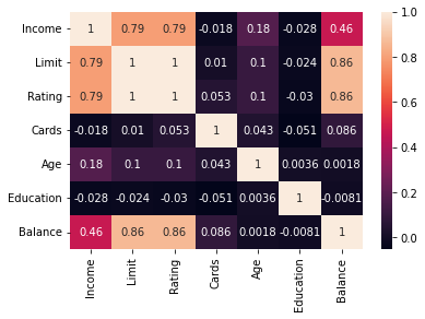
PROBLEM: Which feature is the strongest predictor of Balance in the data?

sns.heatmap(credit.corr(numeric_only = True), annot = True)

<AxesSubplot: >

X = credit[['Rating']]
y = credit['Balance']

PROBLEM: Build a LinearRegression model, determine the Root Mean Squared Error and interpret the slope and intercept.

credit_model = LinearRegression()

credit_model.fit(X, y)

LinearRegression()

In a Jupyter environment, please rerun this cell to show the HTML representation or trust the notebook.
On GitHub, the HTML representation is unable to render, please try loading this page with nbviewer.org.

print(f'The model is y = {credit_model.coef_[0]}x + {credit_model.intercept_}')

The model is y = 2.5662403273433196x + -390.84634178723786

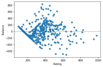
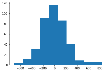
PROBLEM: Examine the residual plot and histogram of residuals. Do they look as they should?

sns.residplot(data = credit, x = X, y = y)

<AxesSubplot: xlabel='Rating', ylabel='Balance'>

plt.hist(y - credit_model.predict(X))

(array([  3.,  11.,  31.,  91., 116.,  86.,  41.,   9.,   6.,   6.]),
 array([-712.2825064 , -558.1506416 , -404.01877679, -249.88691199,
         -95.75504718,   58.37681762,  212.50868243,  366.64054724,
         520.77241204,  674.90427685,  829.03614165]),
 <BarContainer object of 10 artists>)

Other Models

If your goal is more around statistical inference and you want information about things like hypothesis tests on coefficients, the statsmodels library is a more classical statistics interface that also contains a variety of regression models. Below, the OLS model is instantiated, fit, and the results summarized with the .summary() method.

import statsmodels.api as sm

#instantiate the model

#fit it

#summary

#create the intercept term

#fit again

#summary

Typically, we will use the scikitlearn models on our data. Next class will focus on regression models with more features as well as how we can build higher degree polynomial models for our data.