Cross Validation and K-Nearest Neighbors#
Objectives
Use
KNeighborsRegressorto model regression problems using scikitlearnUse
StandardScalerto prepare data for KNN modelsUse
Pipelineto combine the preprocessingUse cross validation to evaluate models
import matplotlib.pyplot as plt
import numpy as np
import pandas as pd
import seaborn as sns

from sklearn.model_selection import train_test_split
from sklearn.pipeline import Pipeline
from sklearn.compose import make_column_transformer
from sklearn.neighbors import KNeighborsRegressor
from sklearn.preprocessing import OneHotEncoder, StandardScaler, PolynomialFeatures
from sklearn.datasets import make_blobs
from sklearn import set_config
set_config('display')
---------------------------------------------------------------------------
ModuleNotFoundError                       Traceback (most recent call last)
Cell In[1], line 4
      2 import numpy as np
      3 import pandas as pd
----> 4 import seaborn as sns
      6 from sklearn.model_selection import train_test_split
      7 from sklearn.pipeline import Pipeline

ModuleNotFoundError: No module named 'seaborn'
A Second Regression Model#
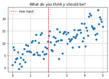
#creating synthetic dataset
x = np.linspace(0, 5, 100)
y = 3*x + 4 + np.random.normal(scale = 3, size = len(x))
df = pd.DataFrame({'x': x, 'y': y})
df.head()
| x | y | |
|---|---|---|
| 0 | 0.000000 | 1.112911 |
| 1 | 0.050505 | 8.442028 |
| 2 | 0.101010 | 7.360462 |
| 3 | 0.151515 | 2.312211 |
| 4 | 0.202020 | 3.587518 |
#plot data and new observation
plt.scatter(x, y)
plt.axvline(2, color='red', linestyle = '--', label = 'new input')
plt.grid()
plt.legend()
plt.title(r'What do you think $y$ should be?');
KNearest Neighbors#
Predict the average of the \(k\) nearest neighbors. One way to think about “nearest” is euclidean distance. We can determine the distance between each data point and the new data point at \(x = 2\) with np.linalg.norm. This is a more general way of determining the euclidean distance between vectors.
#compute distance from each point
#to new observation
df['distance from x = 2'] = np.linalg.norm(df[['x']] - 2, axis = 1)
df.head()
| x | y | distance from x = 2 | |
|---|---|---|---|
| 0 | 0.000000 | 1.112911 | 2.000000 |
| 1 | 0.050505 | 8.442028 | 1.949495 |
| 2 | 0.101010 | 7.360462 | 1.898990 |
| 3 | 0.151515 | 2.312211 | 1.848485 |
| 4 | 0.202020 | 3.587518 | 1.797980 |
#five nearest points
df.nsmallest(5, 'distance from x = 2')
| x | y | distance from x = 2 | |
|---|---|---|---|
| 40 | 2.020202 | 13.137570 | 0.020202 |
| 39 | 1.969697 | 10.641649 | 0.030303 |
| 41 | 2.070707 | 14.921062 | 0.070707 |
| 38 | 1.919192 | 7.956040 | 0.080808 |
| 42 | 2.121212 | 10.442700 | 0.121212 |
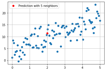
#average of five nearest points
df.nsmallest(5, 'distance from x = 2')['y'].mean()
11.4198040942337
#predicted value with 5 neighbors
plt.scatter(x, y)
plt.plot(2, 11.4198040942337, 'ro', label = 'Prediction with 5 neighbors')
plt.grid()
plt.legend();
Using sklearn#
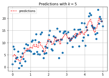
The KNeighborsRegressor estimator can be used to build the KNN model.
from sklearn.neighbors import KNeighborsRegressor
#predict for all data
knn = KNeighborsRegressor(n_neighbors=5)
knn.fit(x.reshape(-1, 1), y)
predictions = knn.predict(x.reshape(-1, 1))
plt.scatter(x, y)
plt.step(x, predictions, '--r', label = 'predictions')
plt.grid()
plt.legend()
plt.title(r'Predictions with $k = 5$');
from ipywidgets import interact
import ipywidgets as widgets
def knn_explorer(n_neighbors):
    knn = KNeighborsRegressor(n_neighbors=n_neighbors)
    knn.fit(x.reshape(-1, 1), y)
    predictions = knn.predict(x.reshape(-1, 1))
    plt.scatter(x, y)
    plt.step(x, predictions, '--r', label = 'predictions')
    plt.grid()
    plt.legend()
    plt.title(f'Predictions with $k = {n_neighbors}$')
    plt.show();
#explore how predictions change as you change k
interact(knn_explorer, n_neighbors = widgets.IntSlider(value = 1,
                                                       low = 1,
                                                       high = len(x)));
KNeighborsRegressor(metric = 'manhattan')
KNeighborsRegressor(metric='manhattan')In a Jupyter environment, please rerun this cell to show the HTML representation or trust the notebook.
On GitHub, the HTML representation is unable to render, please try loading this page with nbviewer.org.
KNeighborsRegressor(metric='manhattan')
Cross Validation#
“Cross-validation is a resampling method that uses different portions of the data to test and train a model on different iterations. It is mainly used in settings where the goal is prediction, and one wants to estimate how accurately a predictive model will perform in practice.” – Wikipedia
In short, this is a way for us to better understand the quality of the predictions made by our estimator.
K-Fold Cross Validation#

from sklearn.model_selection import cross_val_score, cross_val_predict
from sklearn.linear_model import LinearRegression
#linear regression model
lr = LinearRegression()
#knn model
knn = KNeighborsRegressor()
#cross validate linear model
cross_val_score(lr, x.reshape(-1, 1), y)
array([ 0.05002084, -0.13676708, -0.01574163, -0.03091175, 0.02478929])
#cross validate knn model
cross_val_score(knn, x.reshape(-1, 1), y)
array([-1.01619217, -0.29881553, -0.46458949, 0.09059758, -0.39398357])
Exercise: Predicting Bike Riders#
Below a dataset is loaded using the fetch_openml function. The objective is to predict rider count.
from sklearn.datasets import fetch_openml
bikes = fetch_openml(data_id = 44063)
print(bikes.DESCR)
Dataset used in the tabular data benchmark https://github.com/LeoGrin/tabular-benchmark,
                                  transformed in the same way. This dataset belongs to the "regression on categorical and
                                  numerical features" benchmark. Original description:

Bike sharing systems are new generation of traditional bike rentals where whole process from membership, rental and return
back has become automatic. Through these systems, user is able to easily rent a bike from a particular position and return
back at another position. Currently, there are about over 500 bike-sharing programs around the world which is composed of
over 500 thousands bicycles. Today, there exists great interest in these systems due to their important role in traffic,
environmental and health issues.

Apart from interesting real world applications of bike sharing systems, the characteristics of data being generated by
these systems make them attractive for the research. Opposed to other transport services such as bus or subway, the duration
of travel, departure and arrival position is explicitly recorded in these systems. This feature turns bike sharing system into
a virtual sensor network that can be used for sensing mobility in the city. Hence, it is expected that most of important
events in the city could be detected via monitoring these data.

Bike-sharing rental process is highly correlated to the environmental and seasonal settings. For instance, weather conditions,
precipitation, day of week, season, hour of the day, etc. can affect the rental behaviors. The core data set is related to
the two-year historical log corresponding to years 2011 and 2012 from Capital Bikeshare system, Washington D.C., USA which is
publicly available in http://capitalbikeshare.com/system-data. We aggregated the data on two hourly and daily basis and then
extracted and added the corresponding weather and seasonal information. Weather information are extracted from http://www.freemeteo.com.

Use of this dataset in publications must be cited to the following publication:
Fanaee-T, Hadi, and Gama, Joao, "Event labeling combining ensemble detectors and background knowledge",
Progress in Artificial Intelligence (2013): pp. 1-15, Springer Berlin Heidelberg, doi:10.1007/s13748-013-0040-3.

Attributes:
- season : season (1:springer, 2:summer, 3:fall, 4:winter)
- yr : year (0: 2011, 1:2012)
- mnth : month ( 1 to 12)
- hr : hour (0 to 23)
- holiday : weather day is holiday or not (extracted from http://dchr.dc.gov/page/holiday-schedule)
- weekday : day of the week
- workingday : if day is neither weekend nor holiday is 1, otherwise is 0.
- weathersit :
    - 1: Clear, Few clouds, Partly cloudy, Partly cloudy
    - 2: Mist + Cloudy, Mist + Broken clouds, Mist + Few clouds, Mist
    - 3: Light Snow, Light Rain + Thunderstorm + Scattered clouds, Light Rain + Scattered clouds
    - 4: Heavy Rain + Ice Pallets + Thunderstorm + Mist, Snow + Fog
- temp : Normalized temperature in Celsius. The values are divided to 41 (max)
- atemp: Normalized feeling temperature in Celsius. The values are divided to 50 (max)
- hum: Normalized humidity. The values are divided to 100 (max)
- windspeed: Normalized wind speed. The values are divided to 67 (max)
- casual: count of casual users
- registered: count of registered users
- cnt: count of total rental bikes including both casual and registered

This version was cleanup up by Joaquin Vanschoren:
- Category labels replaced by category names (season, weathersit, year)
- Turned back normalization for temperature and windspeed for interpretability
- Renamed features for readability

Downloaded from openml.org.
bikes.frame.info()
<class 'pandas.core.frame.DataFrame'>
RangeIndex: 17379 entries, 0 to 17378
Data columns (total 12 columns):
 #   Column      Non-Null Count  Dtype
---  ------      --------------  -----
 0   season      17379 non-null  category
 1   year        17379 non-null  category
 2   month       17379 non-null  float64
 3   hour        17379 non-null  float64
 4   holiday     17379 non-null  category
 5   workingday  17379 non-null  category
 6   weather     17379 non-null  category
 7   temp        17379 non-null  float64
 8   feel_temp   17379 non-null  float64
 9   humidity    17379 non-null  float64
 10  windspeed   17379 non-null  float64
 11  count       17379 non-null  float64
dtypes: category(5), float64(7)
memory usage: 1.0 MB
data = bikes.frame
data.head()
| season | year | month | hour | holiday | workingday | weather | temp | feel_temp | humidity | windspeed | count | |
|---|---|---|---|---|---|---|---|---|---|---|---|---|
| 0 | 1 | 0 | 1.0 | 0.0 | 0 | 0 | 0 | 9.84 | 14.395 | 0.81 | 0.0 | 16.0 |
| 1 | 1 | 0 | 1.0 | 1.0 | 0 | 0 | 0 | 9.02 | 13.635 | 0.80 | 0.0 | 40.0 |
| 2 | 1 | 0 | 1.0 | 2.0 | 0 | 0 | 0 | 9.02 | 13.635 | 0.80 | 0.0 | 32.0 |
| 3 | 1 | 0 | 1.0 | 3.0 | 0 | 0 | 0 | 9.84 | 14.395 | 0.75 | 0.0 | 13.0 |
| 4 | 1 | 0 | 1.0 | 4.0 | 0 | 0 | 0 | 9.84 | 14.395 | 0.75 | 0.0 | 1.0 |
data['holiday'].value_counts()
0    16879
1      500
Name: holiday, dtype: int64
data['weather'].value_counts()
0    11413
2     4544
3     1419
1        3
Name: weather, dtype: int64
data['holiday'].value_counts()
0    16879
1      500
Name: holiday, dtype: int64
data['season'].value_counts()
0    4496
2    4409
1    4242
3    4232
Name: season, dtype: int64
data['year'].value_counts()
1    8734
0    8645
Name: year, dtype: int64
#split data
X_train, X_test, y_train, y_test = train_test_split(data.drop(columns='count'), data['count'], random_state=42)
X_train.head(2)
| season | year | month | hour | holiday | workingday | weather | temp | feel_temp | humidity | windspeed | |
|---|---|---|---|---|---|---|---|---|---|---|---|
| 1945 | 2 | 0 | 3.0 | 20.0 | 0 | 0 | 2 | 11.48 | 13.635 | 0.45 | 16.9979 |
| 13426 | 0 | 1 | 7.0 | 15.0 | 0 | 1 | 3 | 37.72 | 42.425 | 0.35 | 23.9994 |
#encode categorical features
encoder = make_column_transformer((OneHotEncoder(drop = 'first'), ['season', 'weather']),
                                 remainder = 'passthrough')
#encode categorical features and scale others
encoder = make_column_transformer((OneHotEncoder(drop = 'first'), ['season', 'weather']),
                                 remainder = StandardScaler())
#fit and transform training data
X_train_transformed = encoder.fit_transform(X_train)
#transform test data
X_test_transformed = encoder.transform(X_test)
#linear regression model
lr = LinearRegression()
#cross validate
cross_val_score(lr, X_train_transformed, y_train, cv = 10)
array([0.4179818 , 0.39728929, 0.36351367, 0.38537894, 0.4039477 ,
       0.42911072, 0.3830556 , 0.38717789, 0.39539381, 0.41339759])
#knn model with 5 neighbors
knn = KNeighborsRegressor()
#cross validate
cross_val_score(knn, X_train_transformed, y_train, cv = 10)
array([0.69359044, 0.71116924, 0.66795855, 0.65825036, 0.65512769,
       0.68970725, 0.69961195, 0.66875247, 0.68285728, 0.66897624])
knn.fit(X_train_transformed, y_train)
KNeighborsRegressor()In a Jupyter environment, please rerun this cell to show the HTML representation or trust the notebook.
On GitHub, the HTML representation is unable to render, please try loading this page with nbviewer.org.
KNeighborsRegressor()
knn.score(X_test_transformed, y_test)
0.6957260397958962
Pipeline#
The Pipeline class allows us to combine all the preprocessing and modeling steps together in a single object. Once created, the Pipeline works just like an estimator with a .fit and a .predict and .score method. To access individual steps in the pipeline use the .named_steps attribute of the pipeline.
from sklearn.pipeline import Pipeline
#instantiate pipeline
pipe = Pipeline([('ohe', encoder),
                ('lr', LinearRegression())])
#fit on train
pipe.fit(X_train, y_train)
Pipeline(steps=[('ohe',
                 ColumnTransformer(remainder=StandardScaler(),
                                   transformers=[('onehotencoder',
                                                  OneHotEncoder(drop='first'),
                                                  ['season', 'weather'])])),
                ('lr', LinearRegression())])
In a Jupyter environment, please rerun this cell to show the HTML representation or trust the notebook. On GitHub, the HTML representation is unable to render, please try loading this page with nbviewer.org.
Pipeline(steps=[('ohe',
                 ColumnTransformer(remainder=StandardScaler(),
                                   transformers=[('onehotencoder',
                                                  OneHotEncoder(drop='first'),
                                                  ['season', 'weather'])])),
('lr', LinearRegression())])ColumnTransformer(remainder=StandardScaler(),
transformers=[('onehotencoder', OneHotEncoder(drop='first'),
['season', 'weather'])])['season', 'weather']
OneHotEncoder(drop='first')
['year', 'month', 'hour', 'holiday', 'workingday', 'temp', 'feel_temp', 'humidity', 'windspeed']
StandardScaler()
LinearRegression()
#score on test
pipe.score(X_test, y_test)
0.3952561824510502
#cross validate
cross_val_score(pipe, X_train, y_train, cv = 10)
array([0.4179818 , 0.39728929, 0.36351367, 0.38537894, 0.4039477 ,
       0.42911072, 0.3830556 , 0.38717789, 0.39539381, 0.41339759])
#look at coefficients
pipe.named_steps
{'ohe': ColumnTransformer(remainder=StandardScaler(),
                   transformers=[('onehotencoder', OneHotEncoder(drop='first'),
                                  ['season', 'weather'])]),
 'lr': LinearRegression()}
pipe.named_steps['lr'].coef_
array([  3.15346589,  24.76957468,  68.10547059,  40.44824255,
         8.05398136, -25.02760699,  40.4935775 ,   0.24820152,
        52.18078251,  -4.99252765,   1.04700581,  49.22676167,
        18.03062066, -37.41876958,   3.48330617])
make_column_transformer()
pipe.named_steps['ohe'].get_feature_names_out()
array(['onehotencoder__season_1', 'onehotencoder__season_2',
       'onehotencoder__season_3', 'onehotencoder__weather_1',
       'onehotencoder__weather_2', 'onehotencoder__weather_3',
       'remainder__year', 'remainder__month', 'remainder__hour',
       'remainder__holiday', 'remainder__workingday', 'remainder__temp',
       'remainder__feel_temp', 'remainder__humidity',
       'remainder__windspeed'], dtype=object)
Other Uses of KNN#
Another place the KNeighborsRegressor can be used is to impute missing data. Here, we use the nearest datapoints to fill in missing values. Scikitlearn has a KNNImputer that will fill in missing values based on the average of \(n\) neighbors averages.
from sklearn.impute import KNNImputer
titanic = sns.load_dataset('titanic')
titanic.info()
<class 'pandas.core.frame.DataFrame'>
RangeIndex: 891 entries, 0 to 890
Data columns (total 15 columns):
 #   Column       Non-Null Count  Dtype
---  ------       --------------  -----
 0   survived     891 non-null    int64
 1   pclass       891 non-null    int64
 2   sex          891 non-null    object
 3   age          714 non-null    float64
 4   sibsp        891 non-null    int64
 5   parch        891 non-null    int64
 6   fare         891 non-null    float64
 7   embarked     889 non-null    object
 8   class        891 non-null    category
 9   who          891 non-null    object
 10  adult_male   891 non-null    bool
 11  deck         203 non-null    category
 12  embark_town  889 non-null    object
 13  alive        891 non-null    object
 14  alone        891 non-null    bool
dtypes: bool(2), category(2), float64(2), int64(4), object(5)
memory usage: 80.7+ KB
# instantiate
knn_imputer = KNNImputer()
# fit and transform
titanic['age'] = knn_imputer.fit_transform(titanic[['age']])
titanic.info()
<class 'pandas.core.frame.DataFrame'>
RangeIndex: 891 entries, 0 to 890
Data columns (total 15 columns):
 #   Column       Non-Null Count  Dtype
---  ------       --------------  -----
 0   survived     891 non-null    int64
 1   pclass       891 non-null    int64
 2   sex          891 non-null    object
 3   age          891 non-null    float64
 4   sibsp        891 non-null    int64
 5   parch        891 non-null    int64
 6   fare         891 non-null    float64
 7   embarked     889 non-null    object
 8   class        891 non-null    category
 9   who          891 non-null    object
 10  adult_male   891 non-null    bool
 11  deck         203 non-null    category
 12  embark_town  889 non-null    object
 13  alive        891 non-null    object
 14  alone        891 non-null    bool
dtypes: bool(2), category(2), float64(2), int64(4), object(5)
memory usage: 80.7+ KB
# encoder
encoder = make_column_transformer((KNNImputer(), ['age']),
                                (OneHotEncoder(), ['who', 'embarked', 'class',
                                                   'sex', 'embark_town', 'alive']),
                                 remainder = 'passthrough')
# pipeline
pipe = Pipeline([('imputer', encoder),
                ('knn', KNeighborsRegressor())])
# fit on train
X = titanic.drop(columns=['survived', 'deck'])
y = titanic['survived']
pipe.fit(X, y)
Pipeline(steps=[('imputer',
                 ColumnTransformer(remainder='passthrough',
                                   transformers=[('knnimputer', KNNImputer(),
                                                  ['age']),
                                                 ('onehotencoder',
                                                  OneHotEncoder(),
                                                  ['who', 'embarked', 'class',
                                                   'sex', 'embark_town',
                                                   'alive'])])),
                ('knn', KNeighborsRegressor())])
In a Jupyter environment, please rerun this cell to show the HTML representation or trust the notebook. On GitHub, the HTML representation is unable to render, please try loading this page with nbviewer.org.
Pipeline(steps=[('imputer',
                 ColumnTransformer(remainder='passthrough',
                                   transformers=[('knnimputer', KNNImputer(),
                                                  ['age']),
                                                 ('onehotencoder',
                                                  OneHotEncoder(),
                                                  ['who', 'embarked', 'class',
                                                   'sex', 'embark_town',
                                                   'alive'])])),
('knn', KNeighborsRegressor())])ColumnTransformer(remainder='passthrough',
transformers=[('knnimputer', KNNImputer(), ['age']),
('onehotencoder', OneHotEncoder(),
['who', 'embarked', 'class', 'sex',
'embark_town', 'alive'])])['age']
KNNImputer()
['who', 'embarked', 'class', 'sex', 'embark_town', 'alive']
OneHotEncoder()
['pclass', 'sibsp', 'parch', 'fare', 'adult_male', 'alone']
passthrough
KNeighborsRegressor()
# score on train and test
pipe.score(X, y)
0.642950819672131
cross_val_score(pipe, X, y)
array([0.16466667, 0.32632656, 0.31744183, 0.39640461, 0.47816149])