Reading Files and Split Apply Combine#
This lesson focuses on reviewing our basics with pandas and extending them to more advanced munging and cleaning. Specifically, we will discuss how to load data files, work with missing values, use split-apply-combine, use string methods, and work with string and datetime objects. By the end of this lesson you should feel confident doing basic exploratory data analysis using pandas.
OBJECTIVES
Read local files in as
DataFrameobjectsDrop missing values
Replace missing values
Impute missing values
Use
.groupbyUse built in
.dtmethodsConvert columns to
pd.datetimedatatypeWork with
datetimeobjects in pandas.
Reading Local Files#
To read in a local file, we need to pay close attention to our working directory. This means the current location of your work enviornment with respect to your larger computer filesystem. To find your working directory you can use the os library or if your system executes UNIX commands these can be used.
import os
import numpy as np
import pandas as pd
import matplotlib.pyplot as plt
import seaborn as sns
---------------------------------------------------------------------------
ModuleNotFoundError                       Traceback (most recent call last)
Cell In[1], line 5
      3 import pandas as pd
      4 import matplotlib.pyplot as plt
----> 5 import seaborn as sns

ModuleNotFoundError: No module named 'seaborn'
#pip install seaborn
#check working directory
os.getcwd()
#list all files in directory
os.listdir()
#what's in the data folder?
os.listdir('data')
#what is the path to ufo.csv?
ufo_path = 'data/ufo.csv'
read_csv#
Now, using the path to the ufo.csv file, you can create a DataFrame by passing this filepath to the read_csv function.
#read in ufo data
ufo = pd.read_csv(ufo_path)
# look at first 2 rows
ufo.head(2)
# high level information
ufo.info()
# numerical summaries
ufo.describe()
# categorical summaries
ufo.describe(include = 'object')
# all summaries
ufo.describe(include = 'all')
# tips = sns.load_dataset('tips')
# tips.head()
# tips.describe(include = 'all')
Reading from url#
You can also load datasets from urls where a .csv (or other) file live. Github is one example of this. Note that you want to be sure to use the raw version of the file. For example, a github user dsnair has shared datasets from the book Introduction to Statistical Learning at the link below:
read in the Auto dataset below.
# get url to raw data
auto_url = 'https://raw.githubusercontent.com/dsnair/ISLR/master/data/csv/Auto.csv'
# pass to read_csv
auto = pd.read_csv(auto_url)
#auto.describe?
# look at the first few rows
auto.head(2)
# high level information
auto.info()
Problems#
Read in the
diamonds.csvfile from thedatafolder, and create a DataFrame nameddiamonds.
diamonds_path = 'data/diamonds.csv'
How many diamonds are greater than .5 carat in the data?
What is the highest priced diamond in the data?
Read the data from the
caravan.csvfile in located here. Assign this to a variablecaravan.
How many
Yes’s are in thePurchasecolumn of thecaravandata? No’s?
Missing Values#
Missing values are a common problem in data, whether this is because they are truly missing or there is confusion between the data encoding and the methods you read the data in using.
# re-examine ufo info
ufo.info()
# one-liner to count missing values
ufo.isnull().sum()
# drop missing values
ufo.dropna()
# fill missing values
ufo.fillna('dunno')
# replace missing values with most common value
ufo['Colors Reported'] = ufo['Colors Reported'].fillna(ufo['Colors Reported'].mode()[0])#.isna().sum()
Problem#
Read in the dataset
churn_missing.csvin the data folder, assign to a variablechurnbelow.
Are there any missing values? What columns are they in and how many are there?
What do you think we should do about these? Drop, replace, impute?
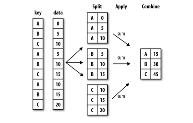
groupby#
Often, you are faced with a dataset that you are interested in summaries within groups based on a condition. The simplest condition is that of a unique value in a single column. Using .groupby you can split your data into unique groups and summarize the results.
NOTE: After splitting you need to summarize!
# sample data
df = pd.DataFrame(
    {
        "A": ["foo", "bar", "foo", "bar", "foo", "bar", "foo", "foo"],
        "B": ["one", "one", "two", "three", "two", "two", "one", "three"],
        "C": np.random.randn(8),
        "D": np.random.randn(8),
    }
)
df
# foo vs. bar
df.groupby('A').mean(numeric_only=True)
# one two or three?
df.groupby('B').mean(numeric_only=True)
# A and B
df.groupby(['A', 'B']).mean(numeric_only=True)
# working with multi-index
df.groupby(['A', 'B'], as_index=False).mean(numeric_only=True)
# age less than 40 survival rate
titanic = sns.load_dataset('titanic')
titanic.groupby(titanic['age'] < 40)[['survived']].mean(numeric_only=True)
Problems#
tips = sns.load_dataset('tips')
tips.head(2)
Average tip for smokers vs. non-smokers.
Average bill by day and time.
What is another question
groupbycan help us answer here?
What does the
as_indexargument do? Demonstrate an example.
Plotting from a DataFrame#
Next class we will introduce two plotting libraries – matplotlib and seaborn. It turns out that a DataFrame also inherits a good bit of matplotlib functionality, and plots can be created directly from a DataFrame.
url = 'https://raw.githubusercontent.com/evorition/astsadata/refs/heads/main/astsadata/data/UnempRate.csv'
unemp = pd.read_csv(url)
#default plot is line
unemp.plot()
unemp.head()
unemp = pd.read_csv(url, index_col = 0)
unemp.head()
unemp.info()
unemp.plot()
unemp.hist()
unemp.boxplot()
#create a new column of shifted measurements
unemp['shifted'] = unemp.shift()
unemp.plot()
unemp.plot(x = 'value', y = 'shifted', kind = 'scatter')
unemp.plot(x = 'value', y = 'shifted', kind = 'scatter', title = 'Unemployment Data', grid = True);
More with pandas and plotting here.
See you Thursday!