Regression Part II

Regression Part II#

OBJECTIVES

Use sklearn to build multiple regression models
Use statsmodels to build multiple regression models
Evaluate models using mean_squared_error
Interpret categorical coefficients

import matplotlib.pyplot as plt
import numpy as np
import pandas as pd
import seaborn as sns

from sklearn.linear_model import LinearRegression
from sklearn.metrics import mean_squared_error

---------------------------------------------------------------------------
ModuleNotFoundError                       Traceback (most recent call last)
Cell In[1], line 4
      2 import numpy as np
      3 import pandas as pd
----> 4 import seaborn as sns
      6 from sklearn.linear_model import LinearRegression
      7 from sklearn.metrics import mean_squared_error

ModuleNotFoundError: No module named 'seaborn'

Using Many Features#

The big idea with a regression model is its ability to learn parameters of linear equations.

\[y = \beta_0 + \beta_1x \quad and \quad y = \beta_0 + \beta_1x_1 + \beta_2x_2 + \beta_3x_3 + \dots\]

\[\begin{split}\begin{bmatrix} 1 & 3.2 & 4 \\ 1 & 5.2 & 3 \\ 1 & 4.1 & 3.4 \end{bmatrix} \begin{bmatrix} \beta_0 \\ \beta_1 \\ \beta_2 \end{bmatrix} = \begin{bmatrix} 12 \\ 10.4 \\ 9.7 \end{bmatrix}\end{split}\]

\[X\beta =y\]

\[\beta = (X^TX)^{-1}X^Ty\]

tips = sns.load_dataset('tips')

X = tips['total_bill'].values.reshape(-1, 1)
y = tips['tip'].values.reshape(-1, 1)

intercept = np.ones(shape = X.shape)
design_matrix = np.concatenate((intercept, X), axis = 1)

design_matrix[:5]

array([[ 1.  , 16.99],
       [ 1.  , 10.34],
       [ 1.  , 21.01],
       [ 1.  , 23.68],
       [ 1.  , 24.59]])

np.linalg.inv(design_matrix.T@design_matrix)@design_matrix.T@y

array([[0.92026961],
       [0.10502452]])

Advertising Data#

The goal here is to predict sales. We have spending on three different media types to help make such predictions. Here, we want to be selective about what features are used as inputs to the model.

ads = pd.read_csv('https://raw.githubusercontent.com/jfkoehler/nyu_bootcamp_fa24/main/data/ads.csv', index_col=0)

ads.head()

	TV	radio	newspaper	sales
1	230.1	37.8	69.2	22.1
2	44.5	39.3	45.1	10.4
3	17.2	45.9	69.3	9.3
4	151.5	41.3	58.5	18.5
5	180.8	10.8	58.4	12.9

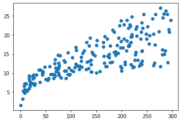
#scatterplot
plt.scatter(ads['TV'], ads['sales']);

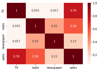
_images/bb21f35f62cb1680cf9fad85468701dae62b59ff836337e69405a034a2a1214a.png

# heatmap
sns.heatmap(ads.corr(), annot = True, cmap = 'Reds');

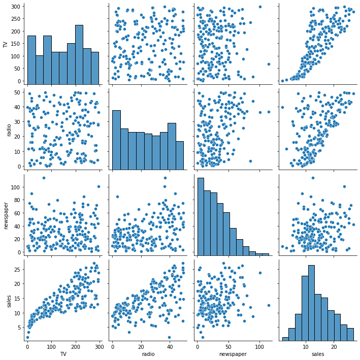
_images/1e61f0be2aeaf35665d95e4f5a895d7e453b35d0445992e3523833c268f6455b.png

# pairplot
sns.pairplot(ads);

_images/86016f8ef7f8221059848c40ec53bafff4769772e788a709275a1cb739643de0.png

Choose a single column as X to predict sales. Justify your choice – remember to make X 2D.

#declare X and y
X = ads[['TV']]
y = ads['sales']

Build a regression model to predict sales using your X above.

# instantiate and fit the model
model1 = LinearRegression().fit(X, y)

Interpret the slope of the model.

# examine slope, what does it mean?
model1.coef_

array([0.04753664])

Interpret the intercept of the model.

#intercept
model1.intercept_

7.032593549127695

Look over the documentation for the mean_squared_error function and use it to evaluate the mean_squared_error of the model.

from sklearn.metrics import mean_squared_error

# MSE
mean_squared_error(y, model1.predict(X))

10.512652915656757

Create baseline predictions using the mean of y.

y.shape

(200,)

np.ones(y.shape).shape

(200,)

y.mean()

14.0225

# ones
baseline = np.ones(y.shape)*y.mean()
# multiply by mean
baseline[:5]

array([14.0225, 14.0225, 14.0225, 14.0225, 14.0225])

mean_squared_error(y, y.mean())

Compute the mean_squared_error of your baseline predictions.

# MSE Baseline
mean_squared_error(y, baseline)

27.085743750000002

Did your model perform better than the baseline?

#Yes!

the `.score` method#

In addition to the mean_squared_error function, you are able to evaluate regression models using the objects .score method. This method evaluates in terms of \(r^2\). One way to understand this metric is as the ratio between the residual sum of squares and the total sum of squares. These are given by:

\[RSS = \sum _{i}(y_{i}-f_{i})^{2}\]

\[TSS = \sum _{i}(y_{i}-{\bar {y}})^{2}\]

and

\[r^2 = 1 - \frac{RSS}{TSS}\]

#model score
model1.score(X, y)

0.611875050850071

You can interpret this as the percent of variation in the data explained by the features according to your model.

Adding Features#

Now, we want to include a second feature as input to the model. Reexamine the plots and correlations above, what is a good second choice?

Choose two columns from the ads data, assign these as X.

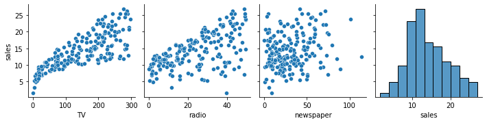
sns.pairplot(ads, y_vars = 'sales')

<seaborn.axisgrid.PairGrid at 0x7fc8cec9cdf0>

_images/4de21f37617b6da0399aa3fc98a5e8d39b8ddc552fed9d5c6e268c092e277b5c.png

# X2
X2 = ads[['TV', 'radio']]

Build a regression model with two features to predict sales.

# lr2 model
model2 = LinearRegression().fit(X2, y)

Evaluate the model using mean_squared_error.

# yhat2
yhat2 = model2.predict(X2)
# MSE
mean_squared_error(y, yhat2)

2.784569900338091

Interpret the coefficients of the model

# make a dataframe here
pd.DataFrame(model2.coef_, index = X2.columns)

	0
TV	0.045755
radio	0.187994

Using `statsmodels`#

A different library for models is the statsmodels library. This contains more classic statistical modeling approaches including a statistical summary of the fit. The interface is slightly different than that of sklearn.

Fit a regression model using statsmodels.

import statsmodels.api as sm

# instantiate and fit
model3 = sm.OLS(y, X2).fit()

Examine the summary of the model using .summary().

# model summary
print(model3.summary())

                                 OLS Regression Results                                
=======================================================================================
Dep. Variable:                  sales   R-squared (uncentered):                   0.981
Model:                            OLS   Adj. R-squared (uncentered):              0.981
Method:                 Least Squares   F-statistic:                              5206.
Date:                Thu, 24 Oct 2024   Prob (F-statistic):                   6.73e-172
Time:                        16:09:34   Log-Likelihood:                         -426.71
No. Observations:                 200   AIC:                                      857.4
Df Residuals:                     198   BIC:                                      864.0
Df Model:                           2                                                  
Covariance Type:            nonrobust                                                  
==============================================================================
                 coef    std err          t      P>|t|      [0.025      0.975]
------------------------------------------------------------------------------
TV             0.0548      0.001     42.962      0.000       0.052       0.057
radio          0.2356      0.008     29.909      0.000       0.220       0.251
==============================================================================
Omnibus:                        6.047   Durbin-Watson:                   2.080
Prob(Omnibus):                  0.049   Jarque-Bera (JB):                8.829
Skew:                          -0.112   Prob(JB):                       0.0121
Kurtosis:                       4.005   Cond. No.                         9.37
==============================================================================

Notes:
[1] R² is computed without centering (uncentered) since the model does not contain a constant.
[2] Standard Errors assume that the covariance matrix of the errors is correctly specified.

Including an intercept term.

# add the constant 
X2 = sm.add_constant(X2)
X2

	const	TV	radio
1	1.0	230.1	37.8
2	1.0	44.5	39.3
3	1.0	17.2	45.9
4	1.0	151.5	41.3
5	1.0	180.8	10.8
...	...	...	...
196	1.0	38.2	3.7
197	1.0	94.2	4.9
198	1.0	177.0	9.3
199	1.0	283.6	42.0
200	1.0	232.1	8.6

200 rows × 3 columns

# fit model
model4 = sm.OLS(y, X2).fit()

# summary
print(model4.summary())

                            OLS Regression Results                            
==============================================================================
Dep. Variable:                  sales   R-squared:                       0.897
Model:                            OLS   Adj. R-squared:                  0.896
Method:                 Least Squares   F-statistic:                     859.6
Date:                Thu, 24 Oct 2024   Prob (F-statistic):           4.83e-98
Time:                        16:13:23   Log-Likelihood:                -386.20
No. Observations:                 200   AIC:                             778.4
Df Residuals:                     197   BIC:                             788.3
Df Model:                           2                                         
Covariance Type:            nonrobust                                         
==============================================================================
                 coef    std err          t      P>|t|      [0.025      0.975]
------------------------------------------------------------------------------
const          2.9211      0.294      9.919      0.000       2.340       3.502
TV             0.0458      0.001     32.909      0.000       0.043       0.048
radio          0.1880      0.008     23.382      0.000       0.172       0.204
==============================================================================
Omnibus:                       60.022   Durbin-Watson:                   2.081
Prob(Omnibus):                  0.000   Jarque-Bera (JB):              148.679
Skew:                          -1.323   Prob(JB):                     5.19e-33
Kurtosis:                       6.292   Cond. No.                         425.
==============================================================================

Notes:
[1] Standard Errors assume that the covariance matrix of the errors is correctly specified.

# LinearRegression()

Example II: Credit Data#

credit = pd.read_csv('https://raw.githubusercontent.com/jfkoehler/nyu_bootcamp_fa24/main/data/Credit.csv', index_col = 0)

credit.head(2)

	Income	Limit	Rating	Cards	Age	Education	Gender	Student	Married	Ethnicity	Balance
1	14.891	3606	283	2	34	11	Male	No	Yes	Caucasian	333
2	106.025	6645	483	3	82	15	Female	Yes	Yes	Asian	903

Build a regression model using Ethnicity feature to predict balance. Interpret the coefficients.

#unique values?
credit['Ethnicity'].unique()

array(['Caucasian', 'Asian', 'African American'], dtype=object)

# using get_dummies
pd.get_dummies(credit['Ethnicity'], drop_first=True)

	Asian	Caucasian
1	0	1
2	1	0
3	1	0
4	1	0
5	0	1
...	...	...
396	0	1
397	0	0
398	0	1
399	0	1
400	1	0

400 rows × 2 columns

Define X and y.

X = pd.get_dummies(credit["Ethnicity"], drop_first=True)
X.head()
y = credit['Balance']

Instantiate and fit.

cat_model = LinearRegression().fit(X, y)

Examine the coefficients.

pd.DataFrame(cat_model.coef_, index = X.columns)

	0
Asian	-18.686275
Caucasian	-12.502513

Interpret the intercept.

cat_model.intercept_

531.0

Mean Squared Error

yhat = cat_model.predict(X)
mean_squared_error(y, yhat, squared=False)

459.13357998933174

Baseline MSE

baseline = np.ones(y.shape)*y.mean()
mean_squared_error(y, baseline, squared=False)

459.18381915633745

cat_model.score(X, y)

0.00021880744304858535

pd.get_dummies(credit, drop_first=True)

	Income	Limit	Rating	Cards	Age	Education	Balance	Gender_Male	Student_Yes	Married_Yes	Ethnicity_Asian	Ethnicity_Caucasian
1	14.891	3606	283	2	34	11	333	1	0	1	0	1
2	106.025	6645	483	3	82	15	903	0	1	1	1	0
3	104.593	7075	514	4	71	11	580	1	0	0	1	0
4	148.924	9504	681	3	36	11	964	0	0	0	1	0
5	55.882	4897	357	2	68	16	331	1	0	1	0	1
...	...	...	...	...	...	...	...	...	...	...	...	...
396	12.096	4100	307	3	32	13	560	1	0	1	0	1
397	13.364	3838	296	5	65	17	480	1	0	0	0	0
398	57.872	4171	321	5	67	12	138	0	0	1	0	1
399	37.728	2525	192	1	44	13	0	1	0	1	0	1
400	18.701	5524	415	5	64	7	966	0	0	0	1	0

400 rows × 12 columns

Problem#

Only using Ethnicity to predict the balance is perhaps too simplistic of a model. Select other features you believe to be important to predicting the Balance and build a regression model using these inputs. Interpret your coefficients and discuss the overall performance of the model.

credit.head()

	Income	Limit	Rating	Cards	Age	Education	Gender	Student	Married	Ethnicity	Balance
1	14.891	3606	283	2	34	11	Male	No	Yes	Caucasian	333
2	106.025	6645	483	3	82	15	Female	Yes	Yes	Asian	903
3	104.593	7075	514	4	71	11	Male	No	No	Asian	580
4	148.924	9504	681	3	36	11	Female	No	No	Asian	964
5	55.882	4897	357	2	68	16	Male	No	Yes	Caucasian	331

X = pd.get_dummies(credit.iloc[:, :-1], drop_first=True)

X.head()

	Income	Limit	Rating	Cards	Age	Education	Gender_Male	Student_Yes	Married_Yes	Ethnicity_Asian	Ethnicity_Caucasian
1	14.891	3606	283	2	34	11	1	0	1	0	1
2	106.025	6645	483	3	82	15	0	1	1	1	0
3	104.593	7075	514	4	71	11	1	0	0	1	0
4	148.924	9504	681	3	36	11	0	0	0	1	0
5	55.882	4897	357	2	68	16	1	0	1	0	1

all_features = LinearRegression().fit(X, y)

yhat = all_features.predict(X)

mean_squared_error(y, yhat, squared=False)

97.2976129033722

all_features.score(X, y)

0.9551015633651758

pd.DataFrame(all_features.coef_, index = X.columns)

	0
Income	-7.803102
Limit	0.190907
Rating	1.136527
Cards	17.724484
Age	-0.613909
Education	-1.098855
Gender_Male	10.653248
Student_Yes	425.747360
Married_Yes	-8.533901
Ethnicity_Asian	16.804179
Ethnicity_Caucasian	10.107025