Inference and Hypothesis Testing

OBJECTIVES

• Review confidence intervals

• Review standard error of the mean

• Introduce Hypothesis Testing

• Hypothesis test with one sample

• Difference in two samples

• Difference in multiple samples

import matplotlib.pyplot as plt
import numpy as np
import pandas as pd
import scipy.stats as stats
import seaborn as sns

---------------------------------------------------------------------------
ModuleNotFoundError                       Traceback (most recent call last)
Cell In[1], line 5
      3 import pandas as pd
      4 import scipy.stats as stats
----> 5 import seaborn as sns

ModuleNotFoundError: No module named 'seaborn'

Why the normal distribution matters

baseball = pd.read_csv('data/baseball.csv', index_col = 0)

baseball.head()

	team	leagueID	player	salary	position	gamesplayed
1	ANA	AL	anderga0	6200000	CF	112
2	ANA	AL	colonba0	11000000	P	3
3	ANA	AL	davanje0	375000	CF	108
4	ANA	AL	donnebr0	375000	P	5
5	ANA	AL	eckstda0	2150000	SS	142

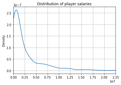
baseball['salary'].plot(kind = 'kde')
plt.xlim(0, baseball['salary'].max())
plt.grid()
plt.title('Distribution of player salaries')

Text(0.5, 1.0, 'Distribution of player salaries')

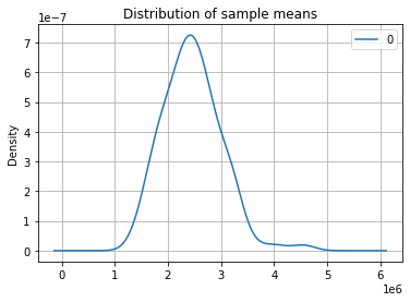
sample_means = []
for _ in range(100):
    sample = baseball['salary'].sample(n = 50)
    sample_mean = sample.mean()
    sample_means.append(sample_mean)

pd.DataFrame(sample_means).plot(kind = 'kde')
plt.xlim()
plt.grid()
plt.title('Distribution of sample means')

Text(0.5, 1.0, 'Distribution of sample means')

Differences between groups

#read in the polls data
polls = pd.read_csv('https://raw.githubusercontent.com/jfkoehler/nyu_bootcamp_fa24/refs/heads/main/data/polls.csv')

#take a peek
polls.head()

	p1	p2	p3	p4	p5
0	5	1	3	5	2
1	1	3	5	5	5
2	2	3	5	3	5
3	4	3	3	3	5
4	5	4	3	2	2

Confidence intervals

\[\mu \pm t_{1 - \alpha / 2} \times \frac{s}{\sqrt{n}}\]

• \(\alpha\): significance level – we determine this

• t: t-score – we look this up

• \(\mu\): we get this from the data

• \(s\): we get this from the data NOTE: This is different than a population standard deviation.

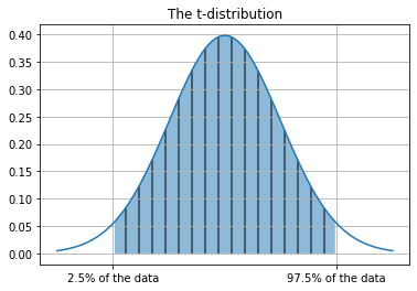
t_dist = stats.t(df = len(polls))
print(t_dist.mean(), t_dist.std())

0.0 1.0067340828210365

x = np.linspace(-3, 3, 100)
plt.plot(x, t_dist.pdf(x))
plt.fill_between(x, t_dist.pdf(x), where = ((x > t_dist.ppf(.025)) &  (x< t_dist.ppf(.975))), hatch = '|', alpha = 0.5)
plt.grid()
plt.title('The t-distribution');
plt.xticks([-2, 2], ['2.5% of the data', '97.5% of the data']);

#examine the first question data
q1 = polls['p1']
q1.head()

0    5
1    1
2    2
3    4
4    5
Name: p1, dtype: int64

#determine degrees of freedom
#i.e. length - 1
dof = len(q1) - 1
print(f'{dof} degrees of freedom')

149 degrees of freedom

#look up test statistic
#we need our alpha and dof
#where do we bound 97.5% of our data
t_stat = stats.t.ppf(1 - 0.05/2, dof)
print(f'The t-statistic is {t_stat}')

The t-statistic is 1.976013177679155

#compute sample standard deviation
s = np.std(q1, ddof = 1)
print(f'The sample standard deviation is {s}')

The sample standard deviation is 1.1317069525271144

#sample size
n = len(q1)
print(f'The sample size is {n}')

The sample size is 150

#compute upper limit
upper = q1.mean() + t_stat*s/np.sqrt(n)
print(f'The upper limit of the confidence interval is {upper}')

The upper limit of the confidence interval is 4.215923838809285

#compute the lower bound
lower = q1.mean() - t_stat*s/np.sqrt(n)
print(f'The lower limit of the confidence interval is {lower}')

The lower limit of the confidence interval is 3.8507428278573816

#print it
(lower, upper)

(3.8507428278573816, 4.215923838809285)

#use scipy
#1 - alpha
#dof
#sem
#(1 - alpha, dof, mean, sem)
stats.t.interval(.95, n - 1, np.mean(q1), stats.sem(q1))

(3.8507428278573816, 4.215923838809285)

#plot it
#take 500 samples of size 7 from poll 1, find mean, kde of the results
sample_means = [q1.sample(20).mean() for _ in range(5000)]
sns.displot(sample_means, kind = 'kde')

<seaborn.axisgrid.FacetGrid at 0x7fd16f36d910>

Problem

• Find the 95% confidence interval for the second poll

• Compare the two intervals, is there much overlap? What does this mean?

q2 = polls['p2']

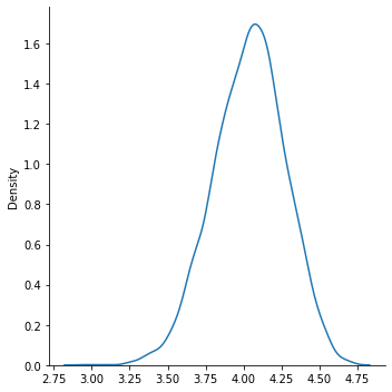
sns.kdeplot(q1)
sns.kdeplot(q2)
plt.title(f'Q1: {q1.mean(): .3f}\nQ2: {q2.mean(): .3f}')

Text(0.5, 1.0, 'Q1:  4.033\nQ2:  3.407')

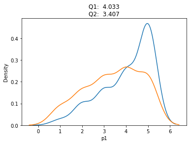
stats.t.interval(.95, n-1, np.mean(q2), stats.sem(q2) )

(3.2001201028191195, 3.613213230514214)

stats.t.interval(.95, n - 1, np.mean(q1), stats.sem(q1))

(3.8507428278573816, 4.215923838809285)

Confidence interval for Difference in Means

In a similar way we can ask questions about the distribution of the difference in means. Here, we construct a confidence interval for the difference between means of the two polls.

#statsmodels imports
from statsmodels.stats.weightstats import CompareMeans, DescrStatsW

#create our objects polls are DescrStatsWeights
#compare means of these
dq1 = DescrStatsW(q1)
dq2 = DescrStatsW(q2)
c = CompareMeans(dq1, dq2)

#90% confidence interval -- represents the difference between 
c.tconfint_diff(.05)

(0.3521083067086064, 0.9012250266247266)

#so what?

Jobs Data

The data below is a sample of job postings from New York City. We want to investigate the lower and upper bound columns.

#read in the data
jobs = pd.read_csv('https://raw.githubusercontent.com/jfkoehler/nyu_bootcamp_fa24/refs/heads/main/data/jobs.csv')

#salary from
jobs.head()

	job_id	title	agency	posting_date	salary_from	salary_to
0	378085	HVAC Service Technic	DEPT OF HEALTH/MENTAL HYGIENE	2018-12-21	385.0	385.0
1	377919	Psychologist, Level	POLICE DEPARTMENT	2018-12-31	62458.0	81131.0
2	379321	Asset Manager	HOUSING PRESERVATION & DVLPMNT	2019-01-07	52524.0	60000.0
3	378658	Public Health Adviso	DEPT OF HEALTH/MENTAL HYGIENE	2019-01-02	37957.0	47142.0
4	321570	Deputy Commissioner,	DEPT OF ENVIRONMENT PROTECTION	2018-01-26	209585.0	209585.0

Margin of Error

Now, the question is to build a confidence interval that achieves a given amount of error.

\[error = z_{\alpha/2} \times \frac{\sigma}{\sqrt{n}}\]

PROBLEM

What is the minimum sample size necessary to estimate the upper salary range with 95% confidence within $3000?

• need \(z\)-score: 1.96

• E: 3000

• \(\sigma\): np.std(jobs['salary_to'])

#do the computation
((1.96*np.std(jobs['salary_to']))/3000)**2

561.6613975822079

#repeat for $500
((1.96*np.std(jobs['salary_to']))/500)**2

20219.81031295948

Testing Significance

Now that we’ve tackled confidence intervals, let’s wrap up with a final test for significance. With a Hypothesis Test, the first step is declaring a null and alternative hypothesis. Typically, this will be an assumption of no difference.

\[H_0: \text{Null Hypothesis}\]

\[H_a: \text{Alternative Hypothesis}\]

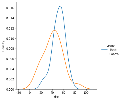
For example, our data below have to do with a reading intervention and assessment after the fact. Our null hypothesis will be:

\[H_0: \mu_1 = \mu_2\]

\[H_a: \mu_1 \neq \mu_2\]

#read in the data
reading = pd.read_csv('https://raw.githubusercontent.com/jfkoehler/nyu_bootcamp_fa24/refs/heads/main/data/DRP.csv')
reading.head()

	id	group	g	drp
0	1	Treat	0	24
1	2	Treat	0	56
2	3	Treat	0	43
3	4	Treat	0	59
4	5	Treat	0	58

#distributions of groups
sns.displot(x = 'drp', hue = 'group', data = reading, kind='kde')

<seaborn.axisgrid.FacetGrid at 0x7fd16fc08fa0>

For our hypothesis test, we need two things:

• Null and alternative hypothesis

\[H_0: \mu_t = \mu_c \]

\[H_a: \mu_t \neq \mu_c \]

• Significance Level

• \(\alpha = 0.05\) Just like before, we will set a tolerance for rejecting the null hypothesis.

#split the groups
treatment = reading.loc[reading['g'] == 0]['drp']
control = reading.loc[reading['g'] == 1]['drp']

#run the test
stats.ttest_ind(treatment, control)

Ttest_indResult(statistic=2.2665515995859433, pvalue=0.02862948283224572)

#alpha at 0.05

SUPPOSE WE WANT TO TEST IF INTERVENTION MADE SCORES HIGHER

\[H_0: \mu_0 = \mu_1\]

\[H_1: \mu_0 < \mu_1\]

#alpha at 0.05

t_score, p = stats.ttest_ind(treatment, control)

p/2

0.01431474141612286

A/B Testing and Proportions

In a similar way, you can test the difference between proportions in groups. For example, consider showing two different ads to samples of 100 customers to see if one encouraged more clicks.

n = 500 #number of views for each
ad1 = 310 #ad1 click
ad2 = 320 #ad2 clicks

from statsmodels.stats.proportion import proportions_ztest
count = np.array([310, 320])
nobs = np.array([500, 500])
stat, pval = proportions_ztest(count, nobs)
print('{0:0.3f}'.format(pval))

0.512

#so what?

PROBLEMS

1. Given the mileage dataset, test the claim on the cars sticker that the average mpg for city driving is 30 mpg.

2. If we increase our food intake, we generally gain weight. In one study, researchers fed 16 non-obese adults, age 25-36 1000 excess calories a day. According to theory, 3500 extra calories will translate into a weight gain of 1 point, therefore we expect each of the subjects to gain 16 pounds. the wtgain dataset contains the before and after eight week period gains.

• Create a new column to represent the weight change of each subject.

• Find the mean and standard deviation for the change.

• Determine the 95% confidence interval for weight change and interpret in complete sentences.

• Test the null hypothesis that the mean weight gain is 16 lbs. What do you conclude?

3. Insurance adjusters are concerned about the high estimates they are receiving from Jocko’s Garage. To see if the estimates are unreasonably high, each of 10 damaged cars was take to Jocko’s and to another garage and the estimates were recorded in the jocko.csv file.

• Create a new column that represents the difference in prices from the two garages. Find the mean and standard deviation of the difference.

• Test the null hypothesis that there is no difference between the estimates at the 0.05 significance level.

mileage_url = 'https://raw.githubusercontent.com/jfkoehler/nyu_bootcamp_fa24/refs/heads/main/data/mileage.csv'
jocko_url = 'https://raw.githubusercontent.com/jfkoehler/nyu_bootcamp_fa24/refs/heads/main/data/JOCKO.csv'
wtgain = 'https://raw.githubusercontent.com/jfkoehler/nyu_bootcamp_fa24/refs/heads/main/data/wtgain.csv'

mileage = pd.read_csv(mileage_url)
mileage.head()

	Car	Mileage
0	1	28.0
1	2	25.7
2	3	25.8
3	4	28.0
4	5	28.5

stats.ttest_1samp(mileage['Mileage'], 30)

TtestResult(statistic=-4.969260253978114, pvalue=0.0001680988457582639, df=15)

mileage.mean()

Car         8.50000
Mileage    28.15625
dtype: float64

weight = pd.read_csv(wtgain)
weight.head(2)

	id	wtb	wta
0	1	55.7	61.7
1	2	54.9	58.8

weight['change'] = weight['wta'] - weight['wtb']
weight.head(2)

	id	wtb	wta	change
0	1	55.7	61.7	6.0
1	2	54.9	58.8	3.9

weight['change'].mean(), weight['change'].std()

(4.73125, 1.7457448267143751)

stats.t.interval(.95,  len(weight) - 1, weight['change'].mean(), stats.sem(weight['change']))

(3.8010082456092764, 5.661491754390724)

stats.ttest_1samp(weight['change'], 16)

TtestResult(statistic=-25.819924716508876, pvalue=7.582374203406457e-14, df=15)

jocko = pd.read_csv(jocko_url)
jocko.head()

	Car	Jocko	Other
0	1	1410	1250
1	2	1550	1300
2	3	1250	1250
3	4	1300	1200
4	5	900	950

jocko['Jocko'].mean() - jocko['Other'].mean()

114.0

stats.ttest_ind(jocko['Jocko'], jocko['Other'])

Ttest_indResult(statistic=0.32060397670781055, pvalue=0.7522026578824064)