Classification II: Logistic Regression#
OBJECTIVES:
Differentiate between Regression and Classification problem settings
Connect Least Squares methods to Classification through Logistic Regression
Interpret coefficients of the model in terms of probabilities
Discuss performance of classification model in terms of accuracy
Understand the effect of an imbalanced target class on model performance
import matplotlib.pyplot as plt
import numpy as np
import pandas as pd
import seaborn as sns
import statsmodels.api as sm
from scipy import stats

from sklearn.linear_model import LinearRegression, LogisticRegression
from sklearn.neighbors import KNeighborsClassifier
from sklearn.preprocessing import StandardScaler, OneHotEncoder
from sklearn.compose import make_column_transformer
from sklearn.model_selection import train_test_split
from sklearn.datasets import load_breast_cancer, load_digits, load_iris
from sklearn.metrics import ConfusionMatrixDisplay
from sklearn.pipeline import Pipeline
Our Motivating Example#
Use the form here while you work through the notebook.
default = pd.read_csv('https://raw.githubusercontent.com/jfkoehler/nyu_bootcamp_fa25/refs/heads/main/data/Default.csv', index_col = 0)
default.info()
<class 'pandas.core.frame.DataFrame'>
Index: 10000 entries, 1 to 10000
Data columns (total 4 columns):
 #   Column   Non-Null Count  Dtype
---  ------   --------------  -----
 0   default  10000 non-null  object
 1   student  10000 non-null  object
 2   balance  10000 non-null  float64
 3   income   10000 non-null  float64
dtypes: float64(2), object(2)
memory usage: 390.6+ KB
default.head(2)
| default | student | balance | income | |
|---|---|---|---|---|
| 1 | No | No | 729.526495 | 44361.625074 |
| 2 | No | Yes | 817.180407 | 12106.134700 |
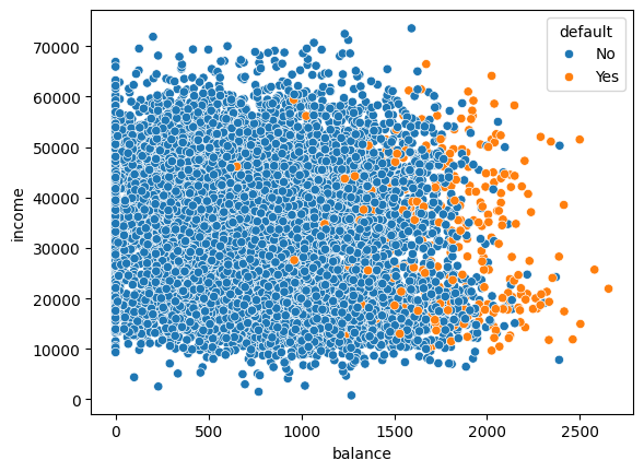
Visualizing Default by Continuous Features#
#scatterplot of balance vs. income colored by default status
sns.scatterplot(data = default, x = 'balance', y = 'income', hue = 'default')
<Axes: xlabel='balance', ylabel='income'>
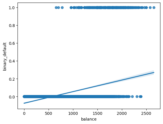
Considering only balance as the predictor#
#create binary default column
default['binary_default'] = np.where(default['default'] == 'No', 0, 1)
#scatter of Balance vs Default
sns.regplot(data = default, x = 'balance', y = 'binary_default')
<Axes: xlabel='balance', ylabel='binary_default'>
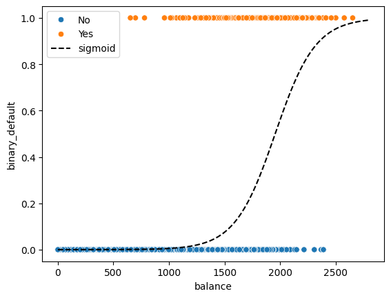
The Sigmoid aka Logistic Function#
#domain
x = np.arange(0, 2800, .1)
sns.scatterplot(data = default, x = 'balance', y = 'binary_default', hue = 'default')
plt.plot(x, 1/(1 + np.exp(-0.0055*x +10.76105259)), '--', color = 'black', label = 'sigmoid')
plt.legend();
def make_plot(m,b):
    sns.scatterplot(data = default, x = 'balance', y = 'binary_default', hue = 'default')
    plt.plot(x, 1/(1 + np.exp(-m*x +b)), '--', color = 'black', label = 'sigmoid')
    plt.legend();
interact(make_plot, m = widgets.FloatSlider(description = r'$\beta_1$', min = 0, max = 0.1, step = 0.001),
         b = widgets.FloatSlider(description = r'$\beta_0$', min = 9, max = 11, step = 0.1));
Example: Hypothetical Models#
Below, the array y represents a target of true values and yhat1 and yhat2 represent two different model predictions. Which model’s predictions are better?
y = np.array([1, 1, 1, 0, 0])
yhat1 = np.array([1, 0, 0, 0, 1])
yhat2 = np.array([1, 1, 1, 1, 0])
pd.DataFrame({'y': y, 'yhat1': yhat1, 'yhat2': yhat2})
| y | yhat1 | yhat2 | |
|---|---|---|---|
| 0 | 1 | 1 | 1 |
| 1 | 1 | 0 | 1 |
| 2 | 1 | 0 | 1 |
| 3 | 0 | 0 | 1 |
| 4 | 0 | 1 | 0 |
Quantifying Loss#
In regression, we understood the LinearRegression model as one seeking to minimize the mean squared error of a linear model with different slope and intercept. With classification, we can also understand the quality of a model given an objective or loss function. One such classification loss functions is log loss and through minimizing this loss with our sigmoid model we get the Logistic Regression model.
from sklearn.metrics import log_loss
log_loss(y, yhat1)
21.626192033470293
log_loss(y, yhat2)
7.20873067782343
Usage should seem familiar#
Fit a LogisticRegression estimator from sklearn on the features:
X = default[['balance']]
y = default['binary_default']
#instantiate
clf = LogisticRegression()
#define X and y
X = default[['balance']]
y = default['default']
#train test split
X_train, X_test, y_train, y_test = train_test_split(X, y, random_state = 22)
#fit on the train
clf.fit(X_train, y_train)
LogisticRegression()In a Jupyter environment, please rerun this cell to show the HTML representation or trust the notebook.
On GitHub, the HTML representation is unable to render, please try loading this page with nbviewer.org.
LogisticRegression()
#examine train and test scores
print(f'Train Accuracy: {clf.score(X_train, y_train)}')
print(f'Test Accuracy: {clf.score(X_test, y_test)}')
Train Accuracy: 0.9728
Test Accuracy: 0.9712
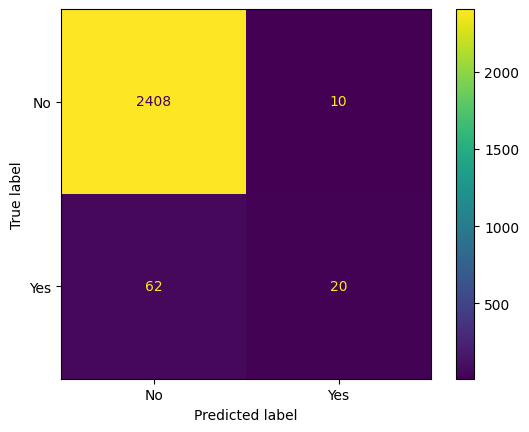
Evaluating the Classifier#
In scikitlearn the primary default evalution metric is accuracy or percent correct. We still need to compare this to our baseline – typically predicting the most frequently occurring class. Further, you can investigate the mistakes made with each class by looking at the Confusion Matrix. A quick visualization of this is had using the ConfusionMatrixDisplay.
#baseline -- most frequently occurring class
y_train.value_counts(normalize = True)
default
No     0.966533
Yes    0.033467
Name: proportion, dtype: float64
from sklearn.metrics import ConfusionMatrixDisplay
#from estimator
ConfusionMatrixDisplay.from_estimator(clf, X_test, y_test)
<sklearn.metrics._plot.confusion_matrix.ConfusionMatrixDisplay at 0x139c00710>
Interpreting Output of the Model#
The version of the logistic we have just developed is actually:
Its output represents probabilities of being labeled the positive class in our example. This means that we can interpret the output of the above function using our parameters, remembering that we used the balance feature to predict default.
def predictor(x):
    line = clf.coef_[0]*x + clf.intercept_
    return np.e**line/(1 + np.e**line)
#predict 1000
predictor(1000)
array([0.00548355])
#predict 2000
predictor(2000)
array([0.58905082])
#estimator has this too
clf.predict_proba(np.array([[1000]]))
/Library/Frameworks/Python.framework/Versions/3.12/lib/python3.12/site-packages/sklearn/base.py:493: UserWarning: X does not have valid feature names, but LogisticRegression was fitted with feature names
  warnings.warn(
array([[0.99451645, 0.00548355]])
clf.predict(np.array([[1000], [2000]]))
/Library/Frameworks/Python.framework/Versions/3.12/lib/python3.12/site-packages/sklearn/base.py:493: UserWarning: X does not have valid feature names, but LogisticRegression was fitted with feature names
  warnings.warn(
array(['No', 'Yes'], dtype=object)
PROBLEM: Given the probability of default below, can you understand what the code is doing? Is the model performance different?
#extracting probability of default from lgr
probability_default = clf.predict_proba(X)[:, 1]
#change the probability threshold to predict yes if greater than 30% probability
new_predictions = np.where(probability_default > .3, 'Yes', 'No')
ConfusionMatrixDisplay.from_predictions(y, new_predictions)
<sklearn.metrics._plot.confusion_matrix.ConfusionMatrixDisplay at 0x1392da9f0>

default.head(2)
| default | student | balance | income | binary_default | |
|---|---|---|---|---|---|
| 1 | No | No | 729.526495 | 44361.625074 | 0 |
| 2 | No | Yes | 817.180407 | 12106.134700 | 0 |
ohe = OneHotEncoder(drop = 'first')
transformer = make_column_transformer((ohe, ['student']),
                                      remainder = StandardScaler())
features = ['balance', 'income', 'student']
X = default.loc[:, features]
y = default['binary_default']
X_train, X_test, y_train, y_test = train_test_split(X, y, random_state=22)
X_train = transformer.fit_transform(X_train)
X_test = transformer.transform(X_test)
clf = LogisticRegression().fit(X_train, y_train)
clf.score(X_train, y_train)
0.9741333333333333
clf.score(X_test, y_test)
0.9712
clf.coef_
array([[-0.66485112, 2.75243435, 0.00621226]])
transformer.get_feature_names_out()
array(['onehotencoder__student_Yes', 'remainder__balance',
       'remainder__income'], dtype=object)
Predictions:
student: yes
balance: 1,500 dollars
income: 40,000 dollars
ex1 = np.array([[1, 1500, 40_000]])
#predict probability
clf.predict_proba(ex1)
array([[0., 1.]])
student: no
balance: 1,500 dollars
income: 40,000 dollars
ex2 = np.array([[0, 1500, 40_000]])
#predict probability
clf.predict_proba(ex2)
array([[0., 1.]])
This is similar to our multicollinearity in regression; we will call it confounding#

Using scikitlearn and its Pipeline#
From the original data, to build a model involved:
One hot or dummy encoding the categorical feature.
Standard Scaling the continuous features
Building Logistic model
we can accomplish this all with the Pipeline, where the first step is a make_column_transformer and the second is a LogisticRegression.
from sklearn.pipeline import Pipeline
from sklearn.compose import make_column_transformer
from sklearn.preprocessing import StandardScaler, OneHotEncoder
X_train, X_test, y_train, y_test = train_test_split(default[['student', 'income', 'balance']], default['default'],
                                                   random_state = 22)
# create OneHotEncoder instance
ohe = OneHotEncoder(drop = 'first')
# create StandardScaler instance
sscaler = StandardScaler()
# make column transformer
transformer = make_column_transformer((ohe, ['student']),
                                     remainder = sscaler,
                                     force_int_remainder_cols=False)
# logistic regressor
clf = LogisticRegression()
# pipeline
pipe = Pipeline([('transform', transformer),
                 ('model', clf)])
# fit it
pipe.fit(X_train, y_train)
Pipeline(steps=[('transform',
                 ColumnTransformer(force_int_remainder_cols=False,
                                   remainder=StandardScaler(),
                                   transformers=[('onehotencoder',
                                                  OneHotEncoder(drop='first'),
                                                  ['student'])])),
                ('model', LogisticRegression())])
In a Jupyter environment, please rerun this cell to show the HTML representation or trust the notebook. On GitHub, the HTML representation is unable to render, please try loading this page with nbviewer.org.
Pipeline(steps=[('transform',
                 ColumnTransformer(force_int_remainder_cols=False,
                                   remainder=StandardScaler(),
                                   transformers=[('onehotencoder',
                                                  OneHotEncoder(drop='first'),
                                                  ['student'])])),
('model', LogisticRegression())])ColumnTransformer(force_int_remainder_cols=False, remainder=StandardScaler(),
transformers=[('onehotencoder', OneHotEncoder(drop='first'),
['student'])])['student']
OneHotEncoder(drop='first')
['income', 'balance']
StandardScaler()
LogisticRegression()
# score on train and test
print(f'Train Score: {pipe.score(X_train, y_train)}')
print(f'Test Score: {pipe.score(X_test, y_test)}')
Train Score: 0.9741333333333333
Test Score: 0.9712
pipe.named_steps['model'].coef_
array([[-0.66485112, 0.00621226, 2.75243435]])
Problem#
Below, a dataset on bank customer churn is loaded and displayed. Your objective is to predict Exited or not. Use CreditScore, Gender, Age, Tenure, and Balance as predictors. Examine the confusion matrix display. Was your classifier better at predicting exits or non-exits?
from sklearn.datasets import fetch_openml
bank_churn = fetch_openml(data_id = 43390).frame
bank_churn.head()
| RowNumber | CustomerId | Surname | CreditScore | Geography | Gender | Age | Tenure | Balance | NumOfProducts | HasCrCard | IsActiveMember | EstimatedSalary | Exited | |
|---|---|---|---|---|---|---|---|---|---|---|---|---|---|---|
| 0 | 1 | 15634602 | Hargrave | 619 | France | Female | 42 | 2 | 0.00 | 1 | 1 | 1 | 101348.88 | 1 |
| 1 | 2 | 15647311 | Hill | 608 | Spain | Female | 41 | 1 | 83807.86 | 1 | 0 | 1 | 112542.58 | 0 |
| 2 | 3 | 15619304 | Onio | 502 | France | Female | 42 | 8 | 159660.80 | 3 | 1 | 0 | 113931.57 | 1 |
| 3 | 4 | 15701354 | Boni | 699 | France | Female | 39 | 1 | 0.00 | 2 | 0 | 0 | 93826.63 | 0 |
| 4 | 5 | 15737888 | Mitchell | 850 | Spain | Female | 43 | 2 | 125510.82 | 1 | 1 | 1 | 79084.10 | 0 |
bank_churn.to_csv('bank_churn.csv')
#create train/test split -- random_state = 11
X = bank_churn.drop(columns = ['Exited', 'RowNumber', 'CustomerId', 'Surname'])
y = bank_churn['Exited']
X_train, X_test, y_train, y_test = train_test_split(X, y, random_state=11)
y_train.value_counts(normalize = True)
Exited
0    0.7976
1    0.2024
Name: proportion, dtype: float64
#make categorical features numeric
ohe = OneHotEncoder(drop = 'first')
#scale numeric features
scale = StandardScaler()
transformer = make_column_transformer((ohe, ['Geography', 'Gender']),
                        remainder=scale)
#pipeline for transform and model with logistic regression
lgr_pipe = Pipeline([('transformer', transformer),
                     ('model', KNeighborsClassifier())])
#fit it
lgr_pipe.fit(X_train, y_train)
#visualize confusion matrix
ConfusionMatrixDisplay.from_estimator(lgr_pipe, X_test, y_test)
<sklearn.metrics._plot.confusion_matrix.ConfusionMatrixDisplay at 0x13d63ab10>
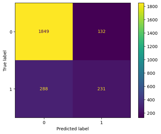
lgr_pipe.score(X_test, y_test)
0.832
Practice#
from sklearn.datasets import load_breast_cancer
cancer = load_breast_cancer(as_frame=True).frame
cancer.head(3)
# use all features
# train/test split -- random_state = 42
# pipeline to scale then knn
# pipeline to scale then logistic
# fit knn
# fit logreg
# compare confusion matrices on test data