Evaluating Classification Models

OBJECTIVES

• Use the confusion matrix to evaluate classification models

• Use precision and recall to evaluate a classifier

• Explore lift and gain to evaluate classifiers

• Determine cost of predicting highest probability targets

import pandas as pd
import numpy as np
import matplotlib.pyplot as plt
from sklearn.linear_model import LogisticRegression
from sklearn.neighbors import KNeighborsClassifier
from sklearn.preprocessing import StandardScaler, OneHotEncoder, PolynomialFeatures
from sklearn.compose import make_column_transformer
from sklearn.metrics import ConfusionMatrixDisplay, confusion_matrix
from sklearn.datasets import load_breast_cancer, load_digits, fetch_openml

Problem

Below, a dataset with information on individuals and whether or not they have heart disease is loaded and displayed. A LogisticRegression and KNeighborsClassifier are used to build predictive models on train/test splits. Examine the confusion matrices and explore the classifiers mistakes.

• Which model do you prefer and why?

• Do you care about predicting each of these classes equally?

• Is there a ratio other than accuracy you think is more important based on the confusion matrix?

heart = fetch_openml(data_id=43823).frame

heart.head()

	Age	Sex	Chest_pain_type	BP	Cholesterol	FBS_over_120	EKG_results	Max_HR	Exercise_angina	ST_depression	Slope_of_ST	Number_of_vessels_fluro	Thallium	Heart_Disease
0	70	1	4	130	322	0	2	109	0	2.4	2	3	3	Presence
1	67	0	3	115	564	0	2	160	0	1.6	2	0	7	Absence
2	57	1	2	124	261	0	0	141	0	0.3	1	0	7	Presence
3	64	1	4	128	263	0	0	105	1	0.2	2	1	7	Absence
4	74	0	2	120	269	0	2	121	1	0.2	1	1	3	Absence

heart.info()

<class 'pandas.core.frame.DataFrame'>
RangeIndex: 270 entries, 0 to 269
Data columns (total 14 columns):
 #   Column                   Non-Null Count  Dtype  
---  ------                   --------------  -----  
 0   Age                      270 non-null    int64  
 1   Sex                      270 non-null    int64  
 2   Chest_pain_type          270 non-null    int64  
 3   BP                       270 non-null    int64  
 4   Cholesterol              270 non-null    int64  
 5   FBS_over_120             270 non-null    int64  
 6   EKG_results              270 non-null    int64  
 7   Max_HR                   270 non-null    int64  
 8   Exercise_angina          270 non-null    int64  
 9   ST_depression            270 non-null    float64
 10  Slope_of_ST              270 non-null    int64  
 11  Number_of_vessels_fluro  270 non-null    int64  
 12  Thallium                 270 non-null    int64  
 13  Heart_Disease            270 non-null    object 
dtypes: float64(1), int64(12), object(1)
memory usage: 29.7+ KB

from sklearn.model_selection import train_test_split, cross_val_score

X = heart.iloc[:, :-1]
y = heart['Heart_Disease']
X_train, X_test, y_train, y_test = train_test_split(X, y, random_state = 11)

#instantiate estimator with appropriate parameters
lgr = None
knn = None

#models require scaling data first
scaler = StandardScaler()

from sklearn.pipeline import Pipeline

#instantiate Pipeline's for each model
lgr_pipe = None
knn_pipe = None

#fit the models on the training data

#plot confusion matrices

# fig, ax = plt.subplots(1, 2, figsize = (20, 5))
# ConfusionMatrixDisplay.from_estimator(lgr_pipe, X_test, y_test, ax = ax[0])
# ConfusionMatrixDisplay.from_estimator(knn_pipe, X_test, y_test, ax = ax[1])

Experimenting with n_neighbors

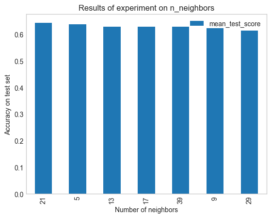
In the example above, we used a single value for k to predict heart disease. As we discussed, different numbers of neighbors may be appropriate in different problems. To experiment with different numbers of neighbors we can use a GridSearchCV to search over different values of k and select the parameters that do the best at predicting on a test set. Below, its use is demonstrated using a single estimator and a pipeline.

from sklearn.model_selection import GridSearchCV

knn = KNeighborsClassifier()
knn.get_params()

{'algorithm': 'auto',
 'leaf_size': 30,
 'metric': 'minkowski',
 'metric_params': None,
 'n_jobs': None,
 'n_neighbors': 5,
 'p': 2,
 'weights': 'uniform'}

params_to_search = {'n_neighbors': [5, 9, 13, 17, 21, 29, 39]}

grid_search = GridSearchCV(estimator=knn, param_grid=params_to_search)

grid_search.fit(X_train, y_train)

GridSearchCV(estimator=KNeighborsClassifier(),
             param_grid={'n_neighbors': [5, 9, 13, 17, 21, 29, 39]})

In a Jupyter environment, please rerun this cell to show the HTML representation or trust the notebook.
On GitHub, the HTML representation is unable to render, please try loading this page with nbviewer.org.

grid_search.best_params_

{'n_neighbors': 21}

results = pd.DataFrame(grid_search.cv_results_)
results.head(1)

	mean_fit_time	std_fit_time	mean_score_time	std_score_time	param_n_neighbors	params	split0_test_score	split1_test_score	split2_test_score	split3_test_score	split4_test_score	mean_test_score	std_test_score	rank_test_score
0	0.004009	0.002808	0.008956	0.005906	5	{'n_neighbors': 5}	0.634146	0.634146	0.7	0.65	0.575	0.638659	0.039961	2

plt.style.use('seaborn-v0_8-whitegrid')
results.sort_values(by = 'mean_test_score', ascending = False).plot(kind = 'bar', x = 'param_n_neighbors', y = 'mean_test_score')
plt.grid()
plt.title('Results of experiment on n_neighbors')
plt.xlabel('Number of neighbors')
plt.ylabel('Accuracy on test set');

knn_pipe = Pipeline([('scale', StandardScaler()), ('knn', KNeighborsClassifier())])
params = {'knn__n_neighbors': [5, 9, 13, 17, 21, 29, 39]}
grid_for_pipeline = GridSearchCV(knn_pipe, param_grid=params)

grid_for_pipeline.fit(X_train, y_train)

GridSearchCV(estimator=Pipeline(steps=[('scale', StandardScaler()),
                                       ('knn', KNeighborsClassifier())]),
             param_grid={'knn__n_neighbors': [5, 9, 13, 17, 21, 29, 39]})

In a Jupyter environment, please rerun this cell to show the HTML representation or trust the notebook.
On GitHub, the HTML representation is unable to render, please try loading this page with nbviewer.org.

grid_for_pipeline.best_params_

{'knn__n_neighbors': 5}

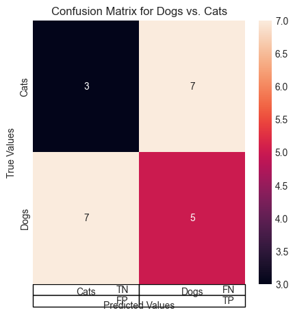
Expanding our metrics

ex = np.array([[3, 7], [7, 5]])
ex

array([[3, 7],
       [7, 5]])

import seaborn as sns

fig, ax = plt.subplots(1, 1, figsize = (5, 5))
sns.heatmap(ex, annot = True, ax = ax)
ax.set_yticks([0.5, 1.5], ['Cats', 'Dogs']);
ax.set_ylabel('True Values')
ax.set_xticks([0.5, 1.5], ['Cats', 'Dogs'])
ax.set_xlabel('Predicted Values')
ax.set_title('Confusion Matrix for Dogs vs. Cats');

ex2 = np.array([['TN', 'FN'], ['FP', 'TP']])
ax.table(ex2)

<matplotlib.table.Table at 0x137945af0>

Problem

In our heart disease example, do you think you care more about predicting the presence of heart disease or the absence of it? As such, which metric is more appropriate, precision or recall? Look back at your confusion matrices and calculate the updated metric – which estimator was better?

What is happening with the code below?

y_train_num = np.where(y_train == 'Presence', 1, 0)
y_test_num = np.where(y_test == 'Presence', 1, 0)

grid_to_select_best_recall = GridSearchCV(knn_pipe, param_grid=params, scoring = 'recall').fit(X_train, y_train_num)
print(f'Best recall: {grid_to_select_best_recall.score(X_test, y_test_num)}')

Best recall: 0.84

grid_to_select_best_precision = GridSearchCV(knn_pipe, param_grid=params, scoring = 'precision').fit(X_train, y_train_num)
print(f'Best precision: {grid_to_select_best_precision.score(X_test, y_test_num)}')

Best precision: 0.7241379310344828

Problem

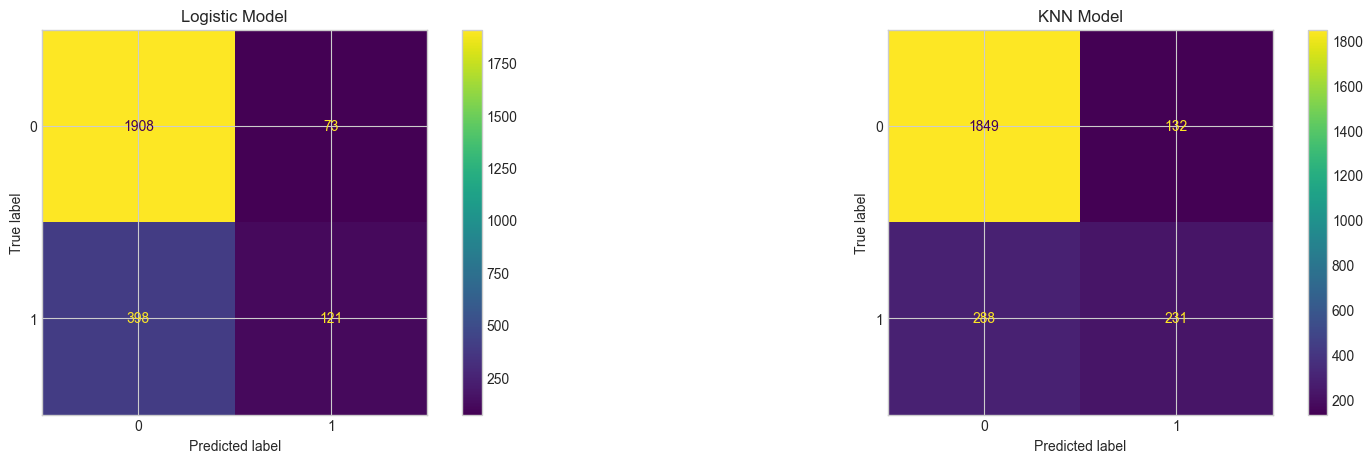
Below, a dataset around customer churn is loaded and displayed. Classification models on the data are given and their confusion matrices.

• Suppose you want to offer an incentive to customers you think are likely to churn, what is an appropriate evaluation metric? Why?

churn = fetch_openml(data_id = 43390).frame

churn.head()

	RowNumber	CustomerId	Surname	CreditScore	Geography	Gender	Age	Tenure	Balance	NumOfProducts	HasCrCard	IsActiveMember	EstimatedSalary	Exited
0	1	15634602	Hargrave	619	France	Female	42	2	0.00	1	1	1	101348.88	1
1	2	15647311	Hill	608	Spain	Female	41	1	83807.86	1	0	1	112542.58	0
2	3	15619304	Onio	502	France	Female	42	8	159660.80	3	1	0	113931.57	1
3	4	15701354	Boni	699	France	Female	39	1	0.00	2	0	0	93826.63	0
4	5	15737888	Mitchell	850	Spain	Female	43	2	125510.82	1	1	1	79084.10	0

import warnings
warnings.filterwarnings('ignore')

X = churn.iloc[:, :-1]
y = churn['Exited']
X.drop(['Surname', 'RowNumber', 'CustomerId'], axis = 1, inplace = True)
X_train, X_test, y_train, y_test = train_test_split(X, y, random_state = 11)

encoder = make_column_transformer((OneHotEncoder(drop = 'first'), ['Geography', 'Gender']),
                                  remainder = StandardScaler())

knn_pipe = Pipeline([('transform', encoder), ('model', KNeighborsClassifier())])
lgr_pipe = Pipeline([('transform', encoder), ('model', LogisticRegression())])

knn_pipe.fit(X_train, y_train)
lgr_pipe.fit(X_train, y_train)

Pipeline(steps=[('transform',
                 ColumnTransformer(remainder=StandardScaler(),
                                   transformers=[('onehotencoder',
                                                  OneHotEncoder(drop='first'),
                                                  ['Geography', 'Gender'])])),
                ('model', LogisticRegression())])

In a Jupyter environment, please rerun this cell to show the HTML representation or trust the notebook.
On GitHub, the HTML representation is unable to render, please try loading this page with nbviewer.org.

#plot confusion matrices
fig, ax = plt.subplots(1, 2, figsize = (20, 5))
ConfusionMatrixDisplay.from_estimator(lgr_pipe, X_test, y_test, ax = ax[0])
ax[0].set_title('Logistic Model')
ConfusionMatrixDisplay.from_estimator(knn_pipe, X_test, y_test, ax = ax[1])
ax[1].set_title('KNN Model');

import ipywidgets as widgets
from ipywidgets import interact
from sklearn.metrics import precision_score, recall_score

def pr_computer(p):
    lgr_pipe = Pipeline([('transform', encoder), ('model', LogisticRegression())])
    lgr_pipe.fit(X_train, y_train)
    ps = lgr_pipe.predict_proba(X_test)[:, 1]
    yhat = np.where(ps > p, 1, 0)
    ConfusionMatrixDisplay.from_predictions(y_test, yhat)
    print(f'Precision {precision_score(y_test, yhat)}\nRecall: {recall_score(y_test, yhat)}')
    plt.show()

interact(pr_computer, p = widgets.FloatSlider(min = 0, max = 1, step = .05))

<function __main__.pr_computer(p)>

PrecisionRecallDisplay

The idea of precision and recall combined with what we saw with changing the probability threshold allows us to understand how precision and recall interact as you run through different probability of positive classes.

from sklearn.metrics import PrecisionRecallDisplay

#plot precision recall curves
fig, ax = plt.subplots(1, 2, figsize = (20, 5))
PrecisionRecallDisplay.from_estimator(lgr_pipe, X_test, y_test, ax = ax[0], plot_chance_level=True)
ax[0].plot(x1, y1, 'ro', label = f'({x1, y1})')

ax[0].set_title('Logistic Model')
PrecisionRecallDisplay.from_estimator(knn_pipe, X_test, y_test, ax = ax[1], plot_chance_level=True)
ax[1].set_title('KNN Model');

Suppose you need to maintain a recall of .6. What kind of precision do you expect?

Predicting Positives

Return to the churn example and a Logistic Regression model on the data.

1. If you were to make predictions on a random 30% of the data, what percent of the true positives would you expect to capture?

2. Use the predict probability capabilities of the estimator to create a DataFrame with the following columns:

probability of prediction = 1	true label
.8	1
.7	1
.4	0

3. Sort the probabilities from largest to smallest. What percentage of the total positives are in the first 3000 rows? What does this tell you about your classifier?

Marketing Problem

Below, a dataset relating to a Portugese Bank Marketing Campaign is loaded and displayed. Your goal is to build a classifier that optimizes to either precision or recall using whichever metric you think is most appropriate. Estimate the lift your classifier has if you were to contact 20% of the customers most likely to subscribe.

bank = fetch_openml(data_id=1461)

print(bank.DESCR)

bank_df = bank.frame

bank_df.head(3)

bank_df.info()

Exit Ticket

Please respond to the questions here.