Evaluating Classification Models

OBJECTIVES

• Use the confusion matrix to evaluate classification models

• Explore precision and recall as evaluation metrics

• Determine cost of predicting highest probability targets

import pandas as pd
import numpy as np
import matplotlib.pyplot as plt
from sklearn.linear_model import LogisticRegression
from sklearn.neighbors import KNeighborsClassifier
from sklearn.preprocessing import StandardScaler, OneHotEncoder, PolynomialFeatures
from sklearn.compose import make_column_transformer
from sklearn.metrics import ConfusionMatrixDisplay, confusion_matrix
from sklearn.datasets import load_breast_cancer, load_digits, fetch_openml

Evaluating Classifiers

Today, we want to think a bit more about the appropriate classification metrics in different situations. Please use this form to summarize your work.

Problem

Below, a dataset with measurements of cancerous and non-cancerous breast tumors is loaded and displayed. Use LogisticRegression and KNeighborsClassifier to build predictive models on train/test splits. Generate a confusion matrix and explore the classifiers mistakes.

• Which model do you prefer and why?

• Do you care about predicting each of these classes equally?

• Is there a ratio other than accuracy you think is more important based on the confusion matrix?

cancer = load_breast_cancer(as_frame=True).frame

cancer.head()

	mean radius	mean texture	mean perimeter	mean area	mean smoothness	mean compactness	mean concavity	mean concave points	mean symmetry	mean fractal dimension	...	worst texture	worst perimeter	worst area	worst smoothness	worst compactness	worst concavity	worst concave points	worst symmetry	worst fractal dimension	target
0	17.99	10.38	122.80	1001.0	0.11840	0.27760	0.3001	0.14710	0.2419	0.07871	...	17.33	184.60	2019.0	0.1622	0.6656	0.7119	0.2654	0.4601	0.11890	0
1	20.57	17.77	132.90	1326.0	0.08474	0.07864	0.0869	0.07017	0.1812	0.05667	...	23.41	158.80	1956.0	0.1238	0.1866	0.2416	0.1860	0.2750	0.08902	0
2	19.69	21.25	130.00	1203.0	0.10960	0.15990	0.1974	0.12790	0.2069	0.05999	...	25.53	152.50	1709.0	0.1444	0.4245	0.4504	0.2430	0.3613	0.08758	0
3	11.42	20.38	77.58	386.1	0.14250	0.28390	0.2414	0.10520	0.2597	0.09744	...	26.50	98.87	567.7	0.2098	0.8663	0.6869	0.2575	0.6638	0.17300	0
4	20.29	14.34	135.10	1297.0	0.10030	0.13280	0.1980	0.10430	0.1809	0.05883	...	16.67	152.20	1575.0	0.1374	0.2050	0.4000	0.1625	0.2364	0.07678	0

5 rows × 31 columns

Problem

Below, a dataset around customer churn is loaded and displayed. Build classification models on the data and visualize the confusion matrix.

• Suppose you want to offer an incentive to customers you think are likely to churn, what is an appropriate evaluation metric?

• Suppose you only have a budget to target 100 individuals you expect to churn. By targeting the most likely predictions to churn, what percent of churned customers did you capture?

churn = fetch_openml(data_id = 43390).frame

churn.head()

	RowNumber	CustomerId	Surname	CreditScore	Geography	Gender	Age	Tenure	Balance	NumOfProducts	HasCrCard	IsActiveMember	EstimatedSalary	Exited
0	1	15634602	Hargrave	619	France	Female	42	2	0.00	1	1	1	101348.88	1
1	2	15647311	Hill	608	Spain	Female	41	1	83807.86	1	0	1	112542.58	0
2	3	15619304	Onio	502	France	Female	42	8	159660.80	3	1	0	113931.57	1
3	4	15701354	Boni	699	France	Female	39	1	0.00	2	0	0	93826.63	0
4	5	15737888	Mitchell	850	Spain	Female	43	2	125510.82	1	1	1	79084.10	0

Problem

Below a dataset containing handwritten digit images is loaded and displayed. Build a classifier to predict 3’s correctly (change it to a binary classification problem).

• Compare the result of the confusion matrix if you use the default probability threshold to one where anything with a 30% chance of being a 3 is labeled a 3.

• How do the confusion matrices change?

• Can you think of a different situation where you might do something like this – changing the prediction threshold?

from sklearn.datasets import load_digits

digits = load_digits(as_frame=True).frame
digits.head(3)

	pixel_0_0	pixel_0_1	pixel_0_2	pixel_0_3	pixel_0_4	pixel_0_5	pixel_0_6	pixel_0_7	pixel_1_0	pixel_1_1	...	pixel_6_7	pixel_7_0	pixel_7_1	pixel_7_2	pixel_7_3	pixel_7_4	pixel_7_5	pixel_7_6	pixel_7_7	target
0	0.0	0.0	5.0	13.0	9.0	1.0	0.0	0.0	0.0	0.0	...	0.0	0.0	0.0	6.0	13.0	10.0	0.0	0.0	0.0	0
1	0.0	0.0	0.0	12.0	13.0	5.0	0.0	0.0	0.0	0.0	...	0.0	0.0	0.0	0.0	11.0	16.0	10.0	0.0	0.0	1
2	0.0	0.0	0.0	4.0	15.0	12.0	0.0	0.0	0.0	0.0	...	0.0	0.0	0.0	0.0	3.0	11.0	16.0	9.0	0.0	2

3 rows × 65 columns

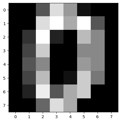
plt.imshow(digits.iloc[0, :-1].values.reshape(8, 8), cmap = 'gray')

<matplotlib.image.AxesImage at 0x1235b9610>

scikit-learn visualizers

• PrecisionRecallDisplay

• ROCurveDisplay

from skplot docs

• plot_cumulative_gain

from sklearn.metrics import PrecisionRecallDisplay, RocCurveDisplay

import scikitplot as skplot