Classification I: Logistic Regression

OBJECTIVES:

• Differentiate between Regression and Classification problem settings

• Connect Least Squares methods to Classification through Logistic Regression

• Interpret coefficients of the model in terms of probabilities

• Discuss performance of classification model in terms of accuracy

• Understand the effect of an imbalanced target class on model performance

import matplotlib.pyplot as plt
import numpy as np
import pandas as pd
import seaborn as sns
import statsmodels.api as sm
from scipy import stats

from sklearn.linear_model import LinearRegression, LogisticRegression
from sklearn.neighbors import KNeighborsClassifier
from sklearn.preprocessing import StandardScaler
from sklearn.model_selection import train_test_split
from sklearn.datasets import load_breast_cancer, load_digits, load_iris

---------------------------------------------------------------------------
ModuleNotFoundError                       Traceback (most recent call last)
Cell In[1], line 4
      2 import numpy as np
      3 import pandas as pd
----> 4 import seaborn as sns
      5 import statsmodels.api as sm
      6 from scipy import stats

ModuleNotFoundError: No module named 'seaborn'

Our Motivating Example

default = pd.read_csv('https://raw.githubusercontent.com/jfkoehler/nyu_bootcamp_fa24/refs/heads/main/data/Default.csv', index_col = 0)

default.info()

<class 'pandas.core.frame.DataFrame'>
Int64Index: 10000 entries, 1 to 10000
Data columns (total 4 columns):
 #   Column   Non-Null Count  Dtype  
---  ------   --------------  -----  
 0   default  10000 non-null  object 
 1   student  10000 non-null  object 
 2   balance  10000 non-null  float64
 3   income   10000 non-null  float64
dtypes: float64(2), object(2)
memory usage: 390.6+ KB

default.head(2)

	default	student	balance	income
1	No	No	729.526495	44361.625074
2	No	Yes	817.180407	12106.134700

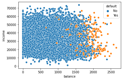
Visualizing Default by Continuous Features

#scatterplot of balance vs. income colored by default status

sns.scatterplot(data = default, x = 'balance', y = 'income', hue = 'default')

<AxesSubplot: xlabel='balance', ylabel='income'>

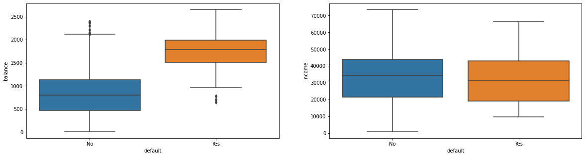
#boxplots for balance and income by default
fig, ax = plt.subplots(1, 2, figsize = (20, 5))
sns.boxplot(data = default, x = 'default', y = 'balance', ax = ax[0])
sns.boxplot(data = default, x = 'default', y = 'income', ax = ax[1])

<AxesSubplot: xlabel='default', ylabel='income'>

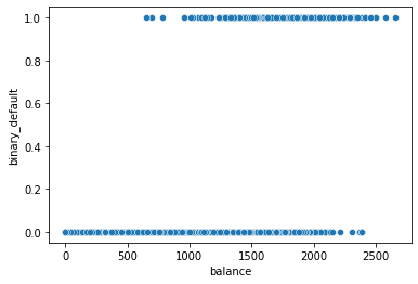
Considering only balance as the predictor

#create binary default column
default['binary_default'] = np.where(default['default'] == 'No', 0, 1)

#scatter of Balance vs Default
sns.scatterplot(data = default, x = 'balance', y = 'binary_default')

<AxesSubplot: xlabel='balance', ylabel='binary_default'>

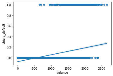
PROBLEM

1. Build a LinearRegression model with balance as the predictor.

2. Interpret the \(r^2\) score and \(rmse\) (root_mean_squared_error) for your regressor.

3. Predict the default for balances: [200, 1000, 1500, 2000, 2500, 3500]. Do these make sense?

X = default[['balance']]
y = default['binary_default']

lr = LinearRegression().fit(X, y)
lr.score(X, y)

0.12258348714904299

from sklearn.metrics import mean_squared_error

np.sqrt(mean_squared_error(y, lr.predict(X)))

0.16806252253551823

new_X = np.array([200, 1000, 1500, 2000, 2500, 3500])

predictions = lr.predict(new_X.reshape(-1, 1))
predictions

/opt/anaconda3/lib/python3.8/site-packages/sklearn/base.py:450: UserWarning: X does not have valid feature names, but LinearRegression was fitted with feature names
  warnings.warn(

array([-0.04921752,  0.05468022,  0.11961631,  0.1845524 ,  0.2494885 ,
        0.37936068])

#regplot
sns.regplot(x = X, y = y)

<AxesSubplot: xlabel='balance', ylabel='binary_default'>

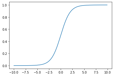
The Sigmoid aka Logistic Function

\[y = \frac{1}{1 + e^{-x}}\]

#define the logistic
def logistic(x): return 1/(1 + np.exp(-x))

#domain
x = np.arange(-10, 10, .1)

#plot it
plt.plot(x, logistic(x))

[<matplotlib.lines.Line2D at 0x7f8f0a43d280>]

Usage should seem familiar

Fit a LogisticRegression estimator from sklearn on the features:

X = default[['balance']]
y = default['binary_default']

#instantiate
clf = LogisticRegression()

#define X and y
X = default[['balance']]
y = default['default']

#train test split
X_train, X_test, y_train, y_test = train_test_split(X, y, random_state = 22)

#fit on the train
clf.fit(X_train, y_train)

LogisticRegression()

In a Jupyter environment, please rerun this cell to show the HTML representation or trust the notebook.
On GitHub, the HTML representation is unable to render, please try loading this page with nbviewer.org.

#examine train and test scores
print(f'Train Score: {clf.score(X_train, y_train)}')
print(f'Test Score: {clf.score(X_test, y_test)}')

Train Score: 0.9728
Test Score: 0.9712

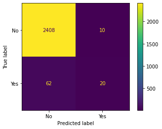
Evaluating the Classifier

In scikitlearn the primary default evalution metric is accuracy or percent correct. We still need to compare this to our baseline – typically predicting the most frequently occurring class. Further, you can investigate the mistakes made with each class by looking at the Confusion Matrix. A quick visualization of this is had using the ConfusionMatrixDisplay.

#baseline -- most frequently occurring class
y_train.value_counts(normalize = True)

No     0.966533
Yes    0.033467
Name: default, dtype: float64

from sklearn.metrics import ConfusionMatrixDisplay

#from estimator
ConfusionMatrixDisplay.from_estimator(clf, X_test, y_test)

<sklearn.metrics._plot.confusion_matrix.ConfusionMatrixDisplay at 0x7f8f26a6c3d0>

Similarities to our earlier work

#there is a coefficient
clf.coef_

array([[0.00556055]])

#there is an intercept
clf.intercept_

array([-10.76105259])

Where was the line?

The version of the logistic we have just developed is actually:

\[ y = \frac{e^{ax + b}}{1 + e^{ax + b}} \]

Its output represents probabilities of being labeled the positive class in our example. This means that we can interpret the output of the above function using our parameters, remembering that we used the balance feature to predict default.

def predictor(x):
    line = clf.coef_[0]*x + clf.intercept_
    return np.e**line/(1 + np.e**line)

#predict 1000
predictor(1000)

array([0.00548355])

#predict 2000
predictor(2000)

array([0.58905082])

#estimator has this too
clf.predict_proba(np.array([[1000]]))

/opt/anaconda3/lib/python3.8/site-packages/sklearn/base.py:450: UserWarning: X does not have valid feature names, but LogisticRegression was fitted with feature names
  warnings.warn(

array([[0.99451645, 0.00548355]])

clf.predict(np.array([[1000]]))

/opt/anaconda3/lib/python3.8/site-packages/sklearn/base.py:450: UserWarning: X does not have valid feature names, but LogisticRegression was fitted with feature names
  warnings.warn(

array(['No'], dtype=object)

Using Categorical Features

default.head(2)

	default	student	balance	income	binary_default
1	No	No	729.526495	44361.625074	0
2	No	Yes	817.180407	12106.134700	0

default['student_binary'] = np.where(default.student == 'No', 0, 1)

X = default[['student_binary']]

#instantiate and fit
clf = LogisticRegression()
clf.fit(X, y)

LogisticRegression()

In a Jupyter environment, please rerun this cell to show the HTML representation or trust the notebook.
On GitHub, the HTML representation is unable to render, please try loading this page with nbviewer.org.

#performance
clf.score(X, y)

0.9667

#coefficients
clf.coef_

array([[0.39960123]])

#compare probabilities
clf.predict_proba(X)

array([[0.97074839, 0.02925161],
       [0.95699704, 0.04300296],
       [0.97074839, 0.02925161],
       ...,
       [0.97074839, 0.02925161],
       [0.97074839, 0.02925161],
       [0.95699704, 0.04300296]])

Using Multiple Features

default.columns

Index(['default', 'student', 'balance', 'income', 'binary_default',
       'student_binary'],
      dtype='object')

features = ['balance', 'income', 'student_binary']
X = default.loc[:, features]
y = default['binary_default']

X_train, X_test, y_train, y_test = train_test_split(X, y, random_state=22)

clf = LogisticRegression().fit(X_train, y_train)

clf.score(X_train, y_train)

0.9674666666666667

clf.score(X_test, y_test)

0.966

Predictions:

• student: yes

• balance: 1,500 dollars

• income: 40,000 dollars

ex1 = np.array([[1500, 40_000, 1]])
#predict probability
clf.predict_proba(ex1)

/opt/anaconda3/lib/python3.8/site-packages/sklearn/base.py:450: UserWarning: X does not have valid feature names, but LogisticRegression was fitted with feature names
  warnings.warn(

array([[0.99774529, 0.00225471]])

• student: no

• balance: 1,500 dollars

• income: 40,000 dollars

ex2 = np.array([[1500, 40_000, 0]])
#predict probability
clf.predict_proba(ex2)

/opt/anaconda3/lib/python3.8/site-packages/sklearn/base.py:450: UserWarning: X does not have valid feature names, but LogisticRegression was fitted with feature names
  warnings.warn(

array([[0.90067473, 0.09932527]])

This is similar to our multicollinearity in regression; we will call it confounding

Using scikitlearn and its Pipeline

From the original data, to build a model involved:

1. One hot or dummy encoding the categorical feature.

2. Standard Scaling the continuous features

3. Building Logistic model

we can accomplish this all with the Pipeline, where the first step is a make_column_transformer and the second is a LogisticRegression.

from sklearn.pipeline import Pipeline 
from sklearn.compose import make_column_transformer
from sklearn.preprocessing import StandardScaler, OneHotEncoder

X_train, X_test, y_train, y_test = train_test_split(default[['student', 'income', 'balance']], default['default'],
                                                   random_state = 22)

# create OneHotEncoder instance
ohe = OneHotEncoder(drop = 'first')

# create StandardScaler instance
sscaler = StandardScaler()

# make column transformer
transformer = make_column_transformer((ohe, ['student']), 
                                     remainder = sscaler)

# logistic regressor
clf = LogisticRegression()

# pipeline
pipe = Pipeline([('transform', transformer), 
                 ('model', clf)])

# fit it
pipe.fit(X_train, y_train)

Pipeline(steps=[('transform',
                 ColumnTransformer(remainder=StandardScaler(),
                                   transformers=[('onehotencoder',
                                                  OneHotEncoder(drop='first'),
                                                  ['student'])])),
                ('model', LogisticRegression())])

In a Jupyter environment, please rerun this cell to show the HTML representation or trust the notebook.
On GitHub, the HTML representation is unable to render, please try loading this page with nbviewer.org.

# score on train and test
print(f'Train Score: {pipe.score(X_train, y_train)}')
print(f'Test Score: {pipe.score(X_test, y_test)}')

Train Score: 0.9741333333333333
Test Score: 0.9712

pipe.named_steps['model'].coef_

array([[-0.66544316,  0.00678331,  2.75262099]])

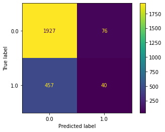
Problem

Below, a dataset on bank customer churn is loaded and displayed. Your objective is to predict Exited or not. Use CreditScore, Gender, Age, Tenure, and Balance as predictors. Examine the confusion matrix display. Was your classifier better at predicting exits or non-exits?

from sklearn.datasets import fetch_openml

bank_churn = fetch_openml(data_id = 43390).frame

bank_churn.head()

	RowNumber	CustomerId	Surname	CreditScore	Geography	Gender	Age	Tenure	Balance	NumOfProducts	HasCrCard	IsActiveMember	EstimatedSalary	Exited
0	1.0	15634602.0	Hargrave	619.0	France	Female	42.0	2.0	0.00	1.0	1.0	1.0	101348.88	1.0
1	2.0	15647311.0	Hill	608.0	Spain	Female	41.0	1.0	83807.86	1.0	0.0	1.0	112542.58	0.0
2	3.0	15619304.0	Onio	502.0	France	Female	42.0	8.0	159660.80	3.0	1.0	0.0	113931.57	1.0
3	4.0	15701354.0	Boni	699.0	France	Female	39.0	1.0	0.00	2.0	0.0	0.0	93826.63	0.0
4	5.0	15737888.0	Mitchell	850.0	Spain	Female	43.0	2.0	125510.82	1.0	1.0	1.0	79084.10	0.0

#create train/test split -- random_state = 42
X = bank_churn[['CreditScore', 'Gender', 'Age', 'Tenure', 'Balance']]
y = bank_churn['Exited']
X_train, X_test, y_train, y_test = train_test_split(X, y, random_state=42)

ohe = OneHotEncoder(drop = 'first')
sscaler = StandardScaler()

#encode gender and standard scale other features
transformer = make_column_transformer((ohe, ['Gender']),
                                     remainder = sscaler)

#set up pipeline to encode/scale and then build logistic regression model
pipe = Pipeline([('transformer', transformer),
                 ('model', LogisticRegression())])

#fit the model on training data
pipe.fit(X_train, y_train)

Pipeline(steps=[('transformer',
                 ColumnTransformer(remainder=StandardScaler(),
                                   transformers=[('onehotencoder',
                                                  OneHotEncoder(drop='first'),
                                                  ['Gender'])])),
                ('model', LogisticRegression())])

In a Jupyter environment, please rerun this cell to show the HTML representation or trust the notebook.
On GitHub, the HTML representation is unable to render, please try loading this page with nbviewer.org.

#score on test and train
print(pipe.score(X_train, y_train))
print(pipe.score(X_test, y_test))

0.7857333333333333
0.7868

y_train.value_counts(normalize = True)

0.0    0.794667
1.0    0.205333
Name: Exited, dtype: float64

#confusion matrix with test data
ConfusionMatrixDisplay.from_estimator(pipe, X_test, y_test)

<sklearn.metrics._plot.confusion_matrix.ConfusionMatrixDisplay at 0x7f8f0af98610>

Compare to KNN and Grid Searching

Let’s compare how this estimator performs compared to the KNeighborsClassifier. This time however, we will be trying many KNN models across different numbers of neighbors. One way we could do this is with a loop; something like:

for neighbor in range(1, 30, 2):
    knn = KNeighborsClassifier(n_neighbors = neighbor).fit(X_train, y_train)

Instead, we can use the GridSearchCV object from sklearn. This will take an estimator and a dictionary with parameters to be searched over.

from sklearn.model_selection import GridSearchCV

# parameters we want to try
params = {'n_neighbors': range(1, 30, 2)}

# estimator with parameters
knn = KNeighborsClassifier()

# grid search object
grid = GridSearchCV(knn, param_grid=params)

# fit it
X = default[['student_binary', 'income', 'balance']]
y = default['default']
grid.fit(X, y)

# what was best?
grid.best_estimator_

# score it 
grid.score(X, y)

Comparing Results

A good way to think about classifier performance is using a confusion matrix. Below, we visualize this using the ConfusionMatrixDisplay.from_estimator.

from sklearn.metrics import ConfusionMatrixDisplay

# a single confusion matrix
ConfusionMatrixDisplay.from_estimator(pipe, X_test, y_test, display_labels=['No', 'Yes'])

# compare knn and logistic
fig, ax = plt.subplots(1, 2, figsize = (19, 5))
ConfusionMatrixDisplay.from_estimator(pipe, X_test, y_test, display_labels=['no', 'yes'], ax = ax[0])
ax[0].set_title('Logistic')
ConfusionMatrixDisplay.from_estimator(grid, X_test, y_test, display_labels=['no', 'yes'], ax = ax[1])
ax[1].set_title('KNN')

Practice

from sklearn.datasets import load_breast_cancer

cancer = load_breast_cancer(as_frame=True).frame

cancer.head(3)

# use all features

# train/test split -- random_state = 42

# pipeline to scale then knn

# pipeline to scale then logistic

# fit knn

# fit logreg

# compare confusion matrices on test data