Introduction to Decision Trees

OBJECTIVES

• Understand how a decision tree is built for classification and regression

• Fit decision tree models using scikit-learn

• Compare and evaluate classifiers

import seaborn as sns
import numpy as np
import pandas as pd
import matplotlib.pyplot as plt

from sklearn.model_selection import train_test_split, GridSearchCV
from sklearn.tree import DecisionTreeClassifier, DecisionTreeRegressor, plot_tree
from sklearn.preprocessing import OneHotEncoder
from sklearn.pipeline import Pipeline
from sklearn.compose import make_column_transformer
from sklearn.metrics import ConfusionMatrixDisplay
from sklearn.inspection import DecisionBoundaryDisplay

---------------------------------------------------------------------------
ModuleNotFoundError                       Traceback (most recent call last)
Cell In[1], line 1
----> 1 import seaborn as sns
      2 import numpy as np
      3 import pandas as pd

ModuleNotFoundError: No module named 'seaborn'

Customer Churn

churn = pd.read_csv('https://raw.githubusercontent.com/jfkoehler/nyu_bootcamp_fa24/refs/heads/main/data/cell_phone_churn.csv')

churn.head()

	state	account_length	area_code	intl_plan	vmail_plan	vmail_message	day_mins	day_calls	day_charge	eve_mins	eve_calls	eve_charge	night_mins	night_calls	night_charge	intl_mins	intl_calls	intl_charge	custserv_calls	churn
0	KS	128	415	no	yes	25	265.1	110	45.07	197.4	99	16.78	244.7	91	11.01	10.0	3	2.70	1	False
1	OH	107	415	no	yes	26	161.6	123	27.47	195.5	103	16.62	254.4	103	11.45	13.7	3	3.70	1	False
2	NJ	137	415	no	no	0	243.4	114	41.38	121.2	110	10.30	162.6	104	7.32	12.2	5	3.29	0	False
3	OH	84	408	yes	no	0	299.4	71	50.90	61.9	88	5.26	196.9	89	8.86	6.6	7	1.78	2	False
4	OK	75	415	yes	no	0	166.7	113	28.34	148.3	122	12.61	186.9	121	8.41	10.1	3	2.73	3	False

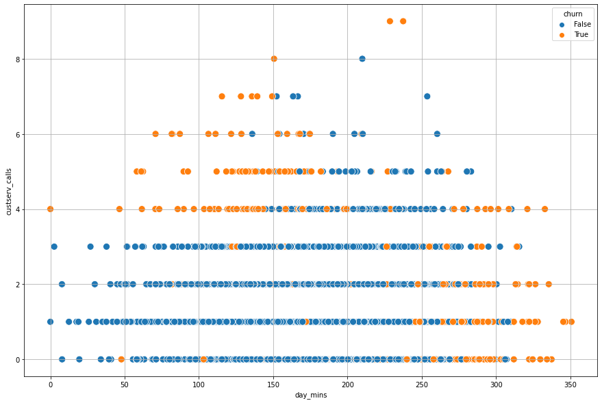
Problem

• Can you determine a value to break the data apart that seperates churn from not churn for the day_mins? What about the custserv_calls?

plt.figure(figsize = (15, 10))
sns.scatterplot(data = churn, x = 'day_mins', y = 'custserv_calls', hue = 'churn', s = 100)
plt.grid();

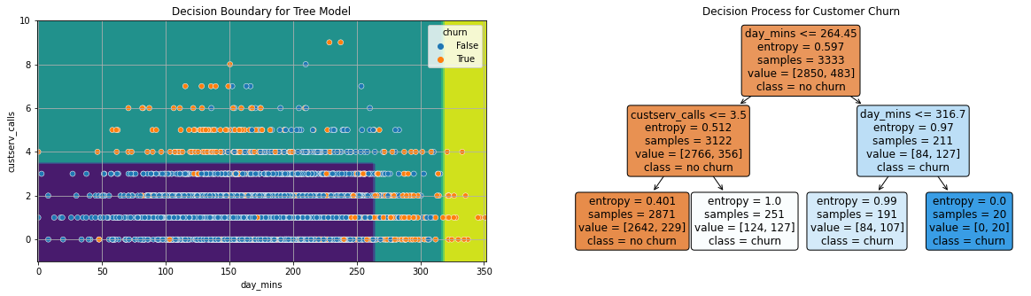
tree = DecisionTreeClassifier(max_depth = 2, criterion='entropy')

X = churn[['day_mins', 'custserv_calls']]
y = churn['churn']

tree.fit(X, y)

DecisionTreeClassifier(criterion='entropy', max_depth=2)

In a Jupyter environment, please rerun this cell to show the HTML representation or trust the notebook.
On GitHub, the HTML representation is unable to render, please try loading this page with nbviewer.org.

fig, ax = plt.subplots(1, 2, figsize = (20, 5))
DecisionBoundaryDisplay.from_estimator(tree, X, ax = ax[0])
sns.scatterplot(data = X, x = 'day_mins', y = 'custserv_calls', hue = y, ax = ax[0])
ax[0].grid()
ax[0].set_title('Decision Boundary for Tree Model');
plot_tree(tree, feature_names=X.columns,
         filled = True,
         fontsize = 12,
         ax = ax[1],
         rounded = True,
         class_names = ['no churn', 'churn'])
ax[1].set_title('Decision Process for Customer Churn');

Titanic Dataset

#load the data
titanic = sns.load_dataset('titanic')
titanic.head(5) #shows first five rows of data

	survived	pclass	sex	age	sibsp	parch	fare	embarked	class	who	adult_male	deck	embark_town	alive	alone
0	0	3	male	22.0	1	0	7.2500	S	Third	man	True	NaN	Southampton	no	False
1	1	1	female	38.0	1	0	71.2833	C	First	woman	False	C	Cherbourg	yes	False
2	1	3	female	26.0	0	0	7.9250	S	Third	woman	False	NaN	Southampton	yes	True
3	1	1	female	35.0	1	0	53.1000	S	First	woman	False	C	Southampton	yes	False
4	0	3	male	35.0	0	0	8.0500	S	Third	man	True	NaN	Southampton	no	True

#subset the data to binary columns
data = titanic.loc[:4, ['alone', 'adult_male', 'survived']]
data

	alone	adult_male	survived
0	False	True	0
1	False	False	1
2	True	False	1
3	False	False	1
4	True	True	0

Suppose you want to use a single column to predict if a passenger survives or not. Which column will do a better job predicting survival in the sample dataset above?

Entropy

One way to quantify the quality of the split is to use a quantity called entropy. This is determined by:

\[H = - \sum p_i \log p_i \]

With a decision tree the idea is to select a feature that produces less entropy.

#all the same -- probability = 1
1*np.log2(1)

0.0

#half and half -- probability = .5
-(1/2*np.log2(1/2) + 1/2*np.log2(1/2))

1.0

#subset the data to age, pclass, and survived five rows
data = titanic.loc[:4, ['age', 'pclass', 'survived']]
data

	age	pclass	survived
0	22.0	3	0
1	38.0	1	1
2	26.0	3	1
3	35.0	1	1
4	35.0	3	0

#compute entropy for pclass
#first class entropy
first_class_entropy = -(2/2*np.log2(2/2))
first_class_entropy

-0.0

#pclass entropy
third_class_entropy = -(1/3*np.log2(1/3) + 2/3*np.log2(2/3))
third_class_entropy

0.9182958340544896

#weighted sum of these
pclass_entropy = 2/5*first_class_entropy + 3/5*third_class_entropy
pclass_entropy

0.5509775004326937

#splitting on age < 30
entropy_left = -(1/2*np.log2(1/2) + 1/2*np.log2(1/2))
entropy_right = -(1/3*np.log2(1/3) + 2/3*np.log2(2/3))
entropy_age = 2/5*entropy_left + 3/5*entropy_right
entropy_age

0.9509775004326937

#original entropy
original_entropy = -((3/5)*np.log2(3/5) + (2/5)*np.log2(2/5))
original_entropy 

0.9709505944546686

# improvement based on pclass
original_entropy - pclass_entropy

0.4199730940219749

#improvement based on age < 30
original_entropy - entropy_age

0.01997309402197489

Using sklearn

The DecisionTreeClassifier can use entropy to build a full decision tree model.

X = data[['age', 'pclass']]
y = data['survived']

from sklearn.tree import DecisionTreeClassifier

#DecisionTreeClassifier?

#instantiate
tree2 = DecisionTreeClassifier(criterion='entropy', max_depth = 1)

#fit
tree2.fit(X, y)

DecisionTreeClassifier(criterion='entropy', max_depth=1)

In a Jupyter environment, please rerun this cell to show the HTML representation or trust the notebook.
On GitHub, the HTML representation is unable to render, please try loading this page with nbviewer.org.

#score it
tree2.score(X, y)

0.8

#predictions
tree2.predict(X)

array([0, 1, 0, 1, 0])

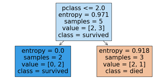
Visualizing the results

The plot_tree function will plot the decision tree model after fitting. There are many options you can use to control the resulting tree drawn.

from sklearn.tree import plot_tree

#plot_tree
fig, ax = plt.subplots(figsize = (10, 5))
plot_tree(tree2, 
          feature_names=X.columns, 
          class_names=['died', 'survived'], filled = True);

PROBLEM

Build a Logistic Regression pipeline to predict purchase.

purchase_data = pd.read_csv('https://raw.githubusercontent.com/YBI-Foundation/Dataset/refs/heads/main/Customer%20Purchase.csv')

purchase_data.head()

	Customer ID	Age	Gender	Education	Review	Purchased
0	1021	30	Female	School	Average	No
1	1022	68	Female	UG	Poor	No
2	1023	70	Female	PG	Good	No
3	1024	72	Female	PG	Good	No
4	1025	16	Female	UG	Average	No

from sklearn.linear_model import LogisticRegression
from sklearn.preprocessing import StandardScaler

encoder = make_column_transformer((OneHotEncoder(), ['Gender', 'Education', 'Review']),
                                 remainder = 'passthrough',
                                 verbose_feature_names_out=False)
model = ''
lgr_pipe = Pipeline([('transform', encoder), ('model', LogisticRegression())])

X = purchase_data.iloc[:, 1:-1]
y = purchase_data['Purchased']

lgr_pipe.fit(X, y)

Pipeline(steps=[('transform',
                 ColumnTransformer(remainder='passthrough',
                                   transformers=[('onehotencoder',
                                                  OneHotEncoder(),
                                                  ['Gender', 'Education',
                                                   'Review'])],
                                   verbose_feature_names_out=False)),
                ('model', LogisticRegression())])

In a Jupyter environment, please rerun this cell to show the HTML representation or trust the notebook.
On GitHub, the HTML representation is unable to render, please try loading this page with nbviewer.org.

lgr_pipe.score(X, y)

0.56

ConfusionMatrixDisplay.from_estimator(lgr_pipe, X, y)

<sklearn.metrics._plot.confusion_matrix.ConfusionMatrixDisplay at 0x7f8f19a97790>

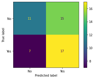
Problem

Build a DecisionTreeClassifier pipeline to predict purchase.

tree_pipe = Pipeline([('transform', encoder), ('model', DecisionTreeClassifier(max_depth = 4))])

tree_pipe.fit(X, y)

Pipeline(steps=[('transform',
                 ColumnTransformer(remainder='passthrough',
                                   transformers=[('onehotencoder',
                                                  OneHotEncoder(),
                                                  ['Gender', 'Education',
                                                   'Review'])],
                                   verbose_feature_names_out=False)),
                ('model', DecisionTreeClassifier(max_depth=4))])

In a Jupyter environment, please rerun this cell to show the HTML representation or trust the notebook.
On GitHub, the HTML representation is unable to render, please try loading this page with nbviewer.org.

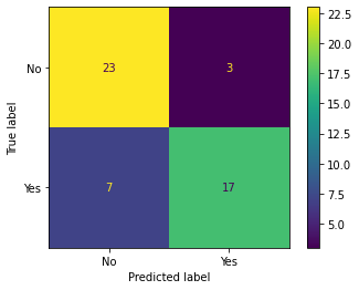
ConfusionMatrixDisplay.from_estimator(tree_pipe, X, y)

<sklearn.metrics._plot.confusion_matrix.ConfusionMatrixDisplay at 0x7f8f1ba593d0>

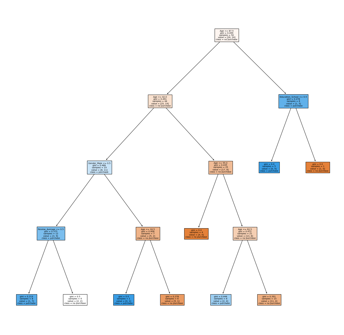
plt.figure(figsize = (20, 20))
plot_tree(tree_pipe['model'], feature_names=tree_pipe['transform'].get_feature_names_out(),
         class_names = ['no purchase', 'purchase'],
         filled = True,
         fontsize=7);

Extra Problem

Suppose you are only able to target 50% of your customers with an advertising incentive. If you only target the highest probability of purchases, which of the models provides the biggest “lift” over the baseline? (Percent of positive purchases) Lift values and argument in slack.

#predict proba for positive class

#sort by probability

#percent of positives on first 50%?

Problem

For next class, read the chapter “Decision Analytic Thinking: What’s a Good Model?” from Data Science for Business. Pay special attention to the cost benefit analysis. You will be asked to use cost/benefit analysis to determine the “best” classifier for an example dataset next class.

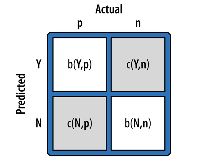
#example cost benefit matrix
cost_benefits = np.array([ [0, -1], [0, 99]])
cost_benefits

array([[ 0, -1],
       [ 0, 99]])

The expected value is computed by:

\[\text{Expected Profit} = p(Y,p)*b(Y, p) + p(N, p)*b(N,p) + p(N,n)*b(N,n) + p(Y,n)*b(Y,n)\]

use this to calculate the expected profit of the Decision Tree and Logistic Regression model. Which is better? Expected Value and argument in slack.

from sklearn.metrics import confusion_matrix

mat = confusion_matrix(y, tree_pipe.predict(X))

mat

array([[23,  3],
       [ 7, 17]])

mat.sum()

50

#expected profit for decision tree model
(((mat/mat.sum())*cost_benefits)).sum()

33.6

lgr_mat = confusion_matrix(y, lgr_pipe.predict(X))

lgr_mat/lgr_mat.sum()

array([[0.22, 0.3 ],
       [0.14, 0.34]])

#expected profit for logistic model
((lgr_mat/lgr_mat.sum())*cost_benefits).sum()

33.36000000000001