Introduction to Decision Trees

OBJECTIVES

• Understand how a decision tree is built for classification and regression

• Fit decision tree models using scikit-learn

• Compare and evaluate classifiers

import seaborn as sns
import numpy as np
import pandas as pd
import matplotlib.pyplot as plt

from sklearn.model_selection import train_test_split, GridSearchCV
from sklearn.tree import DecisionTreeClassifier, DecisionTreeRegressor, plot_tree
from sklearn.preprocessing import OneHotEncoder
from sklearn.pipeline import Pipeline
from sklearn.compose import make_column_transformer
from sklearn.metrics import ConfusionMatrixDisplay
from sklearn.inspection import DecisionBoundaryDisplay

Homework

from sklearn.datasets import fetch_openml
from sklearn.neighbors import KNeighborsClassifier
from sklearn.linear_model import LogisticRegression
from sklearn.tree import DecisionTreeClassifier
from sklearn.model_selection import train_test_split, GridSearchCV
from sklearn.pipeline import Pipeline
from sklearn.preprocessing import StandardScaler, OneHotEncoder
from sklearn.metrics import ConfusionMatrixDisplay
from sklearn.impute import SimpleImputer
from sklearn.compose import make_column_transformer

from sklearn import set_config
set_config(transform_output="pandas")

kidney = fetch_openml(data_id=42972).frame
kidney.head()

	id	age	bp	sg	al	su	rbc	pc	pcc	ba	...	pcv	wc	rc	htn	dm	cad	appet	pe	ane	classification
0	0	48.0	80.0	1.020	1.0	0.0	NaN	normal	notpresent	notpresent	...	44	7800	5.2	yes	yes	no	good	no	no	ckd
1	1	7.0	50.0	1.020	4.0	0.0	NaN	normal	notpresent	notpresent	...	38	6000	NaN	no	no	no	good	no	no	ckd
2	2	62.0	80.0	1.010	2.0	3.0	normal	normal	notpresent	notpresent	...	31	7500	NaN	no	yes	no	poor	no	yes	ckd
3	3	48.0	70.0	1.005	4.0	0.0	normal	abnormal	present	notpresent	...	32	6700	3.9	yes	no	no	poor	yes	yes	ckd
4	4	51.0	80.0	1.010	2.0	0.0	normal	normal	notpresent	notpresent	...	35	7300	4.6	no	no	no	good	no	no	ckd

5 rows × 26 columns

kidney.info()

<class 'pandas.core.frame.DataFrame'>
RangeIndex: 400 entries, 0 to 399
Data columns (total 26 columns):
 #   Column          Non-Null Count  Dtype  
---  ------          --------------  -----  
 0   id              400 non-null    int64  
 1   age             391 non-null    float64
 2   bp              388 non-null    float64
 3   sg              353 non-null    float64
 4   al              354 non-null    float64
 5   su              351 non-null    float64
 6   rbc             248 non-null    object 
 7   pc              335 non-null    object 
 8   pcc             396 non-null    object 
 9   ba              396 non-null    object 
 10  bgr             356 non-null    float64
 11  bu              381 non-null    float64
 12  sc              383 non-null    float64
 13  sod             313 non-null    float64
 14  pot             312 non-null    float64
 15  hemo            348 non-null    float64
 16  pcv             330 non-null    object 
 17  wc              295 non-null    object 
 18  rc              270 non-null    object 
 19  htn             398 non-null    object 
 20  dm              398 non-null    object 
 21  cad             398 non-null    object 
 22  appet           399 non-null    object 
 23  pe              399 non-null    object 
 24  ane             399 non-null    object 
 25  classification  400 non-null    object 
dtypes: float64(11), int64(1), object(14)
memory usage: 81.4+ KB

kidney['rc'] = kidney['rc'].replace({"'t?'":np.nan}).replace("'t43'", np.nan).astype('float')
kidney['pcv'] = kidney['pcv'].replace("'t?'", np.nan).replace("'t43'", np.nan).astype('float')
kidney['wc'] = kidney['wc'].replace("'t6200'", np.nan).replace("'t8400'").replace("'t?'", np.nan).astype('float')

kidney.info()

<class 'pandas.core.frame.DataFrame'>
RangeIndex: 400 entries, 0 to 399
Data columns (total 26 columns):
 #   Column          Non-Null Count  Dtype  
---  ------          --------------  -----  
 0   id              400 non-null    int64  
 1   age             391 non-null    float64
 2   bp              388 non-null    float64
 3   sg              353 non-null    float64
 4   al              354 non-null    float64
 5   su              351 non-null    float64
 6   rbc             248 non-null    object 
 7   pc              335 non-null    object 
 8   pcc             396 non-null    object 
 9   ba              396 non-null    object 
 10  bgr             356 non-null    float64
 11  bu              381 non-null    float64
 12  sc              383 non-null    float64
 13  sod             313 non-null    float64
 14  pot             312 non-null    float64
 15  hemo            348 non-null    float64
 16  pcv             328 non-null    float64
 17  wc              293 non-null    float64
 18  rc              269 non-null    float64
 19  htn             398 non-null    object 
 20  dm              398 non-null    object 
 21  cad             398 non-null    object 
 22  appet           399 non-null    object 
 23  pe              399 non-null    object 
 24  ane             399 non-null    object 
 25  classification  400 non-null    object 
dtypes: float64(14), int64(1), object(11)
memory usage: 81.4+ KB

/var/folders/8v/7bhy8yqn04b7rzqglb2s38200000gn/T/ipykernel_122/1048509165.py:3: FutureWarning: Series.replace without 'value' and with non-dict-like 'to_replace' is deprecated and will raise in a future version. Explicitly specify the new values instead.
  kidney['wc'] = kidney['wc'].replace("'t6200'", np.nan).replace("'t8400'").replace("'t?'", np.nan).astype('float')

cat_cols = kidney.select_dtypes('object').columns.tolist()
cat_cols = cat_cols[:-1]

num_cols = kidney.select_dtypes('number').columns.tolist()


ohe = OneHotEncoder(sparse_output=False)
imp_num = SimpleImputer(strategy = 'mean')
imp_cat = SimpleImputer(strategy = 'most_frequent')
scale = StandardScaler()

imputer = make_column_transformer((imp_num, num_cols),
                             (imp_cat, cat_cols),
                                verbose_feature_names_out=False,
                             remainder = 'passthrough')
ohe = make_column_transformer((ohe, cat_cols),
                              remainder = scale)


X_train, X_test, y_train, y_test = train_test_split(kidney.iloc[:, :-1], kidney.iloc[:, -1])

Customer Churn

churn = pd.read_csv('https://raw.githubusercontent.com/jfkoehler/nyu_bootcamp_fa24/refs/heads/main/data/cell_phone_churn.csv')

churn.head()

	state	account_length	area_code	intl_plan	vmail_plan	vmail_message	day_mins	day_calls	day_charge	eve_mins	eve_calls	eve_charge	night_mins	night_calls	night_charge	intl_mins	intl_calls	intl_charge	custserv_calls	churn
0	KS	128	415	no	yes	25	265.1	110	45.07	197.4	99	16.78	244.7	91	11.01	10.0	3	2.70	1	False
1	OH	107	415	no	yes	26	161.6	123	27.47	195.5	103	16.62	254.4	103	11.45	13.7	3	3.70	1	False
2	NJ	137	415	no	no	0	243.4	114	41.38	121.2	110	10.30	162.6	104	7.32	12.2	5	3.29	0	False
3	OH	84	408	yes	no	0	299.4	71	50.90	61.9	88	5.26	196.9	89	8.86	6.6	7	1.78	2	False
4	OK	75	415	yes	no	0	166.7	113	28.34	148.3	122	12.61	186.9	121	8.41	10.1	3	2.73	3	False

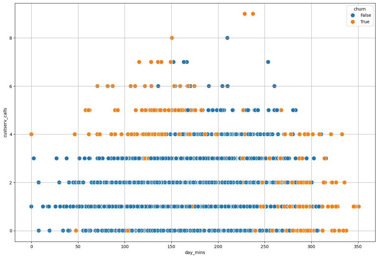
Problem

• Can you determine a value to break the data apart that seperates churn from not churn for the day_mins? What about the custserv_calls?

plt.figure(figsize = (15, 10))
sns.scatterplot(data = churn, x = 'day_mins', y = 'custserv_calls', hue = 'churn', s = 100)
plt.grid();

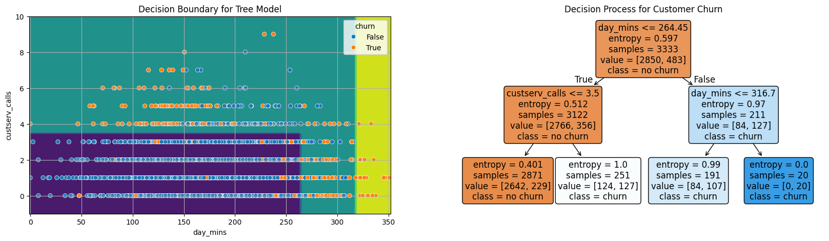
tree = DecisionTreeClassifier(max_depth = 2, criterion='entropy')

X = churn[['day_mins', 'custserv_calls']]
y = churn['churn']

tree.fit(X, y)

DecisionTreeClassifier(criterion='entropy', max_depth=2)

In a Jupyter environment, please rerun this cell to show the HTML representation or trust the notebook.
On GitHub, the HTML representation is unable to render, please try loading this page with nbviewer.org.

fig, ax = plt.subplots(1, 2, figsize = (20, 5))
DecisionBoundaryDisplay.from_estimator(tree, X, ax = ax[0])
sns.scatterplot(data = X, x = 'day_mins', y = 'custserv_calls', hue = y, ax = ax[0])
ax[0].grid()
ax[0].set_title('Decision Boundary for Tree Model');
plot_tree(tree, feature_names=X.columns,
         filled = True,
         fontsize = 12,
         ax = ax[1],
         rounded = True,
         class_names = ['no churn', 'churn'])
ax[1].set_title('Decision Process for Customer Churn');

Titanic Dataset

#load the data
titanic = sns.load_dataset('titanic')
titanic.head(5) #shows first five rows of data

	survived	pclass	sex	age	sibsp	parch	fare	embarked	class	who	adult_male	deck	embark_town	alive	alone
0	0	3	male	22.0	1	0	7.2500	S	Third	man	True	NaN	Southampton	no	False
1	1	1	female	38.0	1	0	71.2833	C	First	woman	False	C	Cherbourg	yes	False
2	1	3	female	26.0	0	0	7.9250	S	Third	woman	False	NaN	Southampton	yes	True
3	1	1	female	35.0	1	0	53.1000	S	First	woman	False	C	Southampton	yes	False
4	0	3	male	35.0	0	0	8.0500	S	Third	man	True	NaN	Southampton	no	True

#subset the data to binary columns
data = titanic.loc[:4, ['alone', 'adult_male', 'survived']]
data

	alone	adult_male	survived
0	False	True	0
1	False	False	1
2	True	False	1
3	False	False	1
4	True	True	0

Suppose you want to use a single column to predict if a passenger survives or not. Which column will do a better job predicting survival in the sample dataset above?

Entropy

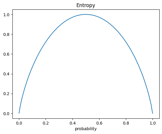
One way to quantify the quality of the split is to use a quantity called entropy. This is determined by:

\[H = - \sum p_i \log p_i \]

With a decision tree the idea is to select a feature that produces less entropy.

#all the same -- probability = 1
1*np.log2(1)

0.0

#half and half -- probability = .5
-(1/2*np.log2(1/2) + 1/2*np.log2(1/2))

1.0

#plot of entropy
def entropy(p):
    return -(p*np.log2(p) + (1-p)*np.log2(1 - p))

p = np.linspace(0.0001, .99999, 100)
plt.plot(p, entropy(p))
plt.title('Entropy')
plt.xlabel('probability');

#subset the data to age, pclass, and survived five rows
data = titanic.loc[:4, ['age', 'pclass', 'survived']]
data

	age	pclass	survived
0	22.0	3	0
1	38.0	1	1
2	26.0	3	1
3	35.0	1	1
4	35.0	3	0

data.loc[data['pclass'] == 1]

	age	pclass	survived
1	38.0	1	1
3	35.0	1	1

#compute entropy for pclass
#first class entropy
first_class_entropy = -(2/2*np.log2(2/2))
first_class_entropy

-0.0

data.loc[data['pclass'] != 1]

	age	pclass	survived
0	22.0	3	0
2	26.0	3	1
4	35.0	3	0

#pclass entropy
third_class_entropy = -(1/3*np.log2(1/3) + 2/3*np.log2(2/3))
third_class_entropy

0.9182958340544896

#weighted sum of these
pclass_entropy = 2/5*first_class_entropy + 3/5*third_class_entropy
pclass_entropy

0.5509775004326937

data

	age	pclass	survived
0	22.0	3	0
1	38.0	1	1
2	26.0	3	1
3	35.0	1	1
4	35.0	3	0

#splitting on age < 30
entropy_left = -(1/2*np.log2(1/2) + 1/2*np.log2(1/2))
entropy_right = -(1/3*np.log2(1/3) + 2/3*np.log2(2/3))
entropy_age = 2/5*entropy_left + 3/5*entropy_right
entropy_age

0.9509775004326937

data

	age	pclass	survived
0	22.0	3	0
1	38.0	1	1
2	26.0	3	1
3	35.0	1	1
4	35.0	3	0

#original entropy
original_entropy = -((3/5)*np.log2(3/5) + (2/5)*np.log2(2/5))
original_entropy 

0.9709505944546686

# improvement based on pclass
original_entropy - pclass_entropy

0.4199730940219749

#improvement based on age < 30
original_entropy - entropy_age

0.01997309402197489

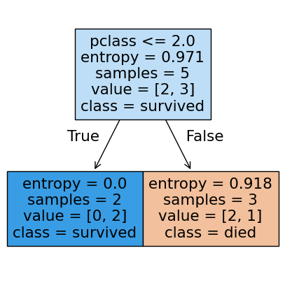
Using sklearn

The DecisionTreeClassifier can use entropy to build a full decision tree model.

X = data[['age', 'pclass']]
y = data['survived']

from sklearn.tree import DecisionTreeClassifier

#DecisionTreeClassifier?

#instantiate
tree2 = DecisionTreeClassifier(criterion='entropy', max_depth = 1)

#fit
tree2.fit(X, y)

DecisionTreeClassifier(criterion='entropy', max_depth=1)

In a Jupyter environment, please rerun this cell to show the HTML representation or trust the notebook.
On GitHub, the HTML representation is unable to render, please try loading this page with nbviewer.org.

#score it
tree2.score(X, y)

0.8

#predictions
tree2.predict(X)

array([0, 1, 0, 1, 0])

Visualizing the results

The plot_tree function will plot the decision tree model after fitting. There are many options you can use to control the resulting tree drawn.

from sklearn.tree import plot_tree

#plot_tree
fig, ax = plt.subplots(figsize = (5,5))
plot_tree(tree2, 
          feature_names=X.columns, 
          class_names=['died', 'survived'], filled = True);

PROBLEM

Build a Logistic Regression and Decision Tree pipeline to predict purchase. Assign the positive predictions probabilities to the variables plgr and ptree respectively.

purchase_data = pd.read_csv('https://raw.githubusercontent.com/jfkoehler/nyu_bootcamp_fa25/refs/heads/main/data/bank-direct-marketing-campaigns.csv')

purchase_data.head()

	age	job	marital	education	default	housing	loan	contact	month	day_of_week	campaign	pdays	previous	poutcome	emp.var.rate	cons.price.idx	cons.conf.idx	euribor3m	nr.employed	y
0	56	housemaid	married	basic.4y	no	no	no	telephone	may	mon	1	999	0	nonexistent	1.1	93.994	-36.4	4.857	5191.0	no
1	57	services	married	high.school	unknown	no	no	telephone	may	mon	1	999	0	nonexistent	1.1	93.994	-36.4	4.857	5191.0	no
2	37	services	married	high.school	no	yes	no	telephone	may	mon	1	999	0	nonexistent	1.1	93.994	-36.4	4.857	5191.0	no
3	40	admin.	married	basic.6y	no	no	no	telephone	may	mon	1	999	0	nonexistent	1.1	93.994	-36.4	4.857	5191.0	no
4	56	services	married	high.school	no	no	yes	telephone	may	mon	1	999	0	nonexistent	1.1	93.994	-36.4	4.857	5191.0	no

purchase_data.info()

<class 'pandas.core.frame.DataFrame'>
RangeIndex: 41188 entries, 0 to 41187
Data columns (total 20 columns):
 #   Column          Non-Null Count  Dtype  
---  ------          --------------  -----  
 0   age             41188 non-null  int64  
 1   job             41188 non-null  object 
 2   marital         41188 non-null  object 
 3   education       41188 non-null  object 
 4   default         41188 non-null  object 
 5   housing         41188 non-null  object 
 6   loan            41188 non-null  object 
 7   contact         41188 non-null  object 
 8   month           41188 non-null  object 
 9   day_of_week     41188 non-null  object 
 10  campaign        41188 non-null  int64  
 11  pdays           41188 non-null  int64  
 12  previous        41188 non-null  int64  
 13  poutcome        41188 non-null  object 
 14  emp.var.rate    41188 non-null  float64
 15  cons.price.idx  41188 non-null  float64
 16  cons.conf.idx   41188 non-null  float64
 17  euribor3m       41188 non-null  float64
 18  nr.employed     41188 non-null  float64
 19  y               41188 non-null  object 
dtypes: float64(5), int64(4), object(11)
memory usage: 6.3+ MB

cat_cols = purchase_data.select_dtypes('object').columns.tolist()
cat_cols

['job',
 'marital',
 'education',
 'default',
 'housing',
 'loan',
 'contact',
 'month',
 'day_of_week',
 'poutcome',
 'y']

cat_cols.remove('y')

cat_cols

['job',
 'marital',
 'education',
 'default',
 'housing',
 'loan',
 'contact',
 'month',
 'day_of_week',
 'poutcome']

from sklearn.linear_model import LogisticRegression
from sklearn.preprocessing import StandardScaler
from sklearn.neighbors import KNeighborsClassifier

encoder = make_column_transformer((OneHotEncoder(sparse_output=False), cat_cols),
                                 remainder = StandardScaler(),
                                 verbose_feature_names_out=False)

knn_pipe = Pipeline([('transform', encoder), ('model', KNeighborsClassifier(n_neighbors=3))])

X = purchase_data.iloc[:, :-1]
y = purchase_data['y']

X_train, X_test, y_train, y_test = train_test_split(X, y, random_state=11, stratify = y)

knn_pipe.fit(X, y)

/Library/Frameworks/Python.framework/Versions/3.12/lib/python3.12/site-packages/sklearn/compose/_column_transformer.py:1623: FutureWarning: 
The format of the columns of the 'remainder' transformer in ColumnTransformer.transformers_ will change in version 1.7 to match the format of the other transformers.
At the moment the remainder columns are stored as indices (of type int). With the same ColumnTransformer configuration, in the future they will be stored as column names (of type str).
To use the new behavior now and suppress this warning, use ColumnTransformer(force_int_remainder_cols=False).

  warnings.warn(

Pipeline(steps=[('transform',
                 ColumnTransformer(remainder=StandardScaler(),
                                   transformers=[('onehotencoder',
                                                  OneHotEncoder(sparse_output=False),
                                                  ['job', 'marital',
                                                   'education', 'default',
                                                   'housing', 'loan', 'contact',
                                                   'month', 'day_of_week',
                                                   'poutcome'])],
                                   verbose_feature_names_out=False)),
                ('model', KNeighborsClassifier(n_neighbors=3))])

In a Jupyter environment, please rerun this cell to show the HTML representation or trust the notebook.
On GitHub, the HTML representation is unable to render, please try loading this page with nbviewer.org.

knn_pipe.score(X, y)

0.9249295911430514

y.value_counts(normalize = True)

y
no     0.887346
yes    0.112654
Name: proportion, dtype: float64

ConfusionMatrixDisplay.from_estimator(knn_pipe, X, y)

<sklearn.metrics._plot.confusion_matrix.ConfusionMatrixDisplay at 0x135b6f0e0>

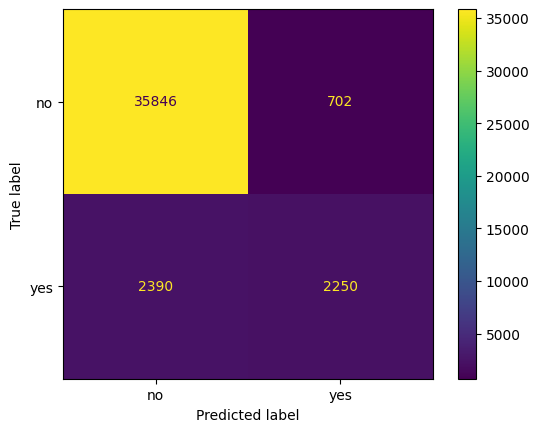
prob_positive = knn_pipe.predict_proba(X)[:, 1]
prob_positive

array([0.        , 0.        , 0.        , ..., 0.33333333, 0.33333333,
       0.66666667])

results = pd.DataFrame({'y': y, 'prob_pos': prob_positive})

results.head()

	y	prob_pos
0	no	0.0
1	no	0.0
2	no	0.0
3	no	0.0
4	no	0.0

results = results.sort_values(by = 'prob_pos', ascending = False)
results.reset_index(inplace = True, drop = True)

results.head()

	y	prob_pos
0	yes	1.0
1	yes	1.0
2	yes	1.0
3	yes	1.0
4	yes	1.0

results.iloc[:41188//10, :]['y'].value_counts()

y
yes    2634
no     1484
Name: count, dtype: int64

y.value_counts()

y
no     36548
yes     4640
Name: count, dtype: int64

2634/4640

0.5676724137931034

results.iloc[:(41188//10)*2, :]['y'].value_counts()

y
no     4265
yes    3971
Name: count, dtype: int64

3971/4640

0.8558189655172413

What does it mean? If we use our model to contact 20% of the most probable to subscribe customers, we would be able to target 85% of the positives.

Problem

Build a DecisionTreeClassifier pipeline to predict purchase, grid searching max_depth parameter. Is this better than the knn model in terms of lift when constrained to the 20% most likely customers to churn.

tree_pipe = Pipeline([('transform', encoder), ('model', DecisionTreeClassifier())])
params = {'model__max_depth': [1, 2, 3, 4, 5, 6, 7]} #fill in the appropriate parameter
tree_grid = GridSearchCV(tree_pipe, param_grid=params)

tree_grid.fit(X_train, y_train)

/Library/Frameworks/Python.framework/Versions/3.12/lib/python3.12/site-packages/sklearn/compose/_column_transformer.py:1623: FutureWarning: 
The format of the columns of the 'remainder' transformer in ColumnTransformer.transformers_ will change in version 1.7 to match the format of the other transformers.
At the moment the remainder columns are stored as indices (of type int). With the same ColumnTransformer configuration, in the future they will be stored as column names (of type str).
To use the new behavior now and suppress this warning, use ColumnTransformer(force_int_remainder_cols=False).

  warnings.warn(

GridSearchCV(estimator=Pipeline(steps=[('transform',
                                        ColumnTransformer(remainder=StandardScaler(),
                                                          transformers=[('onehotencoder',
                                                                         OneHotEncoder(sparse_output=False),
                                                                         ['job',
                                                                          'marital',
                                                                          'education',
                                                                          'default',
                                                                          'housing',
                                                                          'loan',
                                                                          'contact',
                                                                          'month',
                                                                          'day_of_week',
                                                                          'poutcome'])],
                                                          verbose_feature_names_out=False)),
                                       ('model', DecisionTreeClassifier())]),
             param_grid={'model__max_depth': [1, 2, 3, 4, 5, 6, 7]})

In a Jupyter environment, please rerun this cell to show the HTML representation or trust the notebook.
On GitHub, the HTML representation is unable to render, please try loading this page with nbviewer.org.

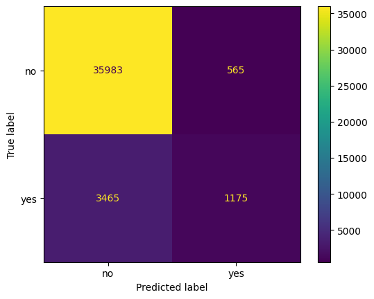
ConfusionMatrixDisplay.from_estimator(tree_grid, X, y)

<sklearn.metrics._plot.confusion_matrix.ConfusionMatrixDisplay at 0x13593ba10>

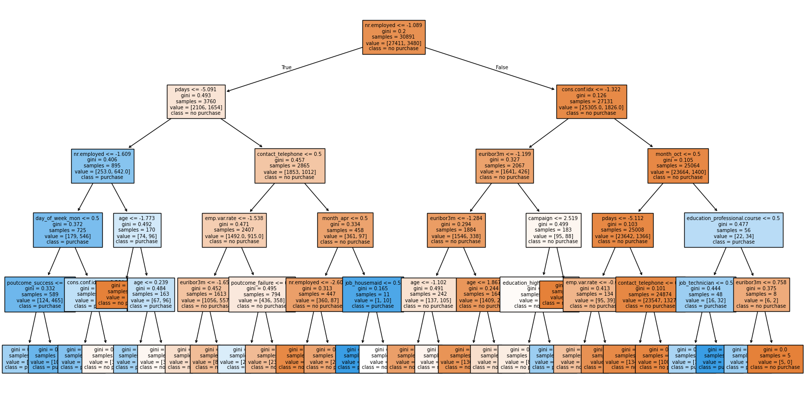
plt.figure(figsize = (20, 10))
plot_tree(tree_grid.best_estimator_['model'], feature_names=tree_pipe['transform'].get_feature_names_out(),
         class_names = ['no purchase', 'purchase'],
         filled = True,
         fontsize=7);

Problem

For next class, read the chapter “Decision Analytic Thinking: What’s a Good Model?” from Data Science for Business. Pay special attention to the cost benefit analysis. You will be asked to use cost/benefit analysis to determine the “best” classifier for an example dataset next class.

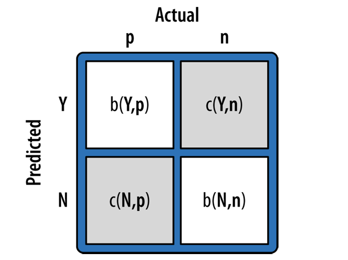
#example cost benefit matrix
cost_benefits = np.array([ [0, -1], [0, 99]])
cost_benefits

array([[ 0, -1],
       [ 0, 99]])

The expected value is computed by:

\[\text{Expected Profit} = p(Y,p)*b(Y, p) + p(N, p)*b(N,p) + p(N,n)*b(N,n) + p(Y,n)*b(Y,n)\]

use this to calculate the expected profit of the Decision Tree and KNN Regression model. Which is better? Expected Value and argument in slack.

from sklearn.metrics import confusion_matrix

mat = confusion_matrix(y, tree_grid.predict(X))

mat

array([[35983,   565],
       [ 3465,  1175]])

mat.sum()

41188

mat/mat.sum()

array([[0.87362824, 0.01371759],
       [0.08412644, 0.02852773]])

(mat/mat.sum())*cost_benefits

array([[ 0.        , -0.01371759],
       [ 0.        ,  2.82424493]])

#expected profit for decision tree model
(((mat/mat.sum())*cost_benefits)).sum()

2.810527338059629

knn_mat = confusion_matrix(y, knn_pipe.predict(X))

knn_mat/knn_mat.sum()

array([[0.87030203, 0.0170438 ],
       [0.05802661, 0.05462756]])

#expected profit for logistic model
((knn_mat/knn_mat.sum())*cost_benefits).sum()

5.391084781975333

EXIT TICKET: here