Boosted Ensembles#
Continuing on with our work with classifiers and ensembles today we introduce boosted models, a powerful collection of tree based models that learn in sequence.
# !pip install xgboost
import numpy as np
import pandas as pd
import matplotlib.pyplot as plt
from sklearn.linear_model import LogisticRegression
from sklearn.pipeline import Pipeline
from sklearn.preprocessing import StandardScaler, OneHotEncoder
from sklearn.compose import make_column_transformer
from sklearn.model_selection import train_test_split
Gradient Boosted Models#

from sklearn.ensemble import HistGradientBoostingClassifier, HistGradientBoostingRegressor
from xgboost import XGBClassifier, XGBRegressor
from sklearn.datasets import fetch_california_housing, load_breast_cancer
from sklearn.datasets import fetch_openml
bikes = fetch_openml("Bike_Sharing_Demand", version=2, as_frame=True).frame
bikes.head()
| season | year | month | hour | holiday | weekday | workingday | weather | temp | feel_temp | humidity | windspeed | count | |
|---|---|---|---|---|---|---|---|---|---|---|---|---|---|
| 0 | spring | 0 | 1 | 0 | False | 6 | False | clear | 9.84 | 14.395 | 0.81 | 0.0 | 16 |
| 1 | spring | 0 | 1 | 1 | False | 6 | False | clear | 9.02 | 13.635 | 0.80 | 0.0 | 40 |
| 2 | spring | 0 | 1 | 2 | False | 6 | False | clear | 9.02 | 13.635 | 0.80 | 0.0 | 32 |
| 3 | spring | 0 | 1 | 3 | False | 6 | False | clear | 9.84 | 14.395 | 0.75 | 0.0 | 13 |
| 4 | spring | 0 | 1 | 4 | False | 6 | False | clear | 9.84 | 14.395 | 0.75 | 0.0 | 1 |
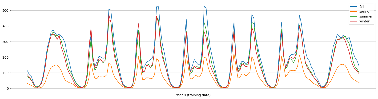
df = bikes[bikes['year'] == 0]
fig,ax = plt.subplots(figsize = (20, 5))
average_bike_rentals = df.groupby(
    ["year", "season", "weekday", "hour"], observed=True
).mean(numeric_only=True)["count"]
average_bike_rentals.groupby(['season'], observed = True).plot(legend = True)
plt.xticks([], [])
plt.xlabel('Year 0 (training data)')
plt.grid();
bikes.info()
<class 'pandas.core.frame.DataFrame'>
RangeIndex: 17379 entries, 0 to 17378
Data columns (total 13 columns):
 #   Column      Non-Null Count  Dtype
---  ------      --------------  -----
 0   season      17379 non-null  category
 1   year        17379 non-null  int64
 2   month       17379 non-null  int64
 3   hour        17379 non-null  int64
 4   holiday     17379 non-null  category
 5   weekday     17379 non-null  int64
 6   workingday  17379 non-null  category
 7   weather     17379 non-null  category
 8   temp        17379 non-null  float64
 9   feel_temp   17379 non-null  float64
 10  humidity    17379 non-null  float64
 11  windspeed   17379 non-null  float64
 12  count       17379 non-null  int64
dtypes: category(4), float64(4), int64(5)
memory usage: 1.3 MB
X = bikes.drop(columns = 'count')
y = bikes['count']
train = bikes[bikes['year'] == 0]
test = bikes[bikes['year'] == 1]
X_train = train.drop(columns = 'count')
y_train = train['count']
X_test = test.drop(columns = 'count')
y_test = test['count']
reg = XGBRegressor(enable_categorical=True)
reg.fit(X_train, y_train)
XGBRegressor(base_score=None, booster=None, callbacks=None,
             colsample_bylevel=None, colsample_bynode=None,
             colsample_bytree=None, device=None, early_stopping_rounds=None,
             enable_categorical=True, eval_metric=None, feature_types=None,
             gamma=None, grow_policy=None, importance_type=None,
             interaction_constraints=None, learning_rate=None, max_bin=None,
             max_cat_threshold=None, max_cat_to_onehot=None,
             max_delta_step=None, max_depth=None, max_leaves=None,
             min_child_weight=None, missing=nan, monotone_constraints=None,
             multi_strategy=None, n_estimators=None, n_jobs=None,
             num_parallel_tree=None, random_state=None, ...)
In a Jupyter environment, please rerun this cell to show the HTML representation or trust the notebook. On GitHub, the HTML representation is unable to render, please try loading this page with nbviewer.org.
XGBRegressor(base_score=None, booster=None, callbacks=None,
             colsample_bylevel=None, colsample_bynode=None,
             colsample_bytree=None, device=None, early_stopping_rounds=None,
             enable_categorical=True, eval_metric=None, feature_types=None,
             gamma=None, grow_policy=None, importance_type=None,
             interaction_constraints=None, learning_rate=None, max_bin=None,
             max_cat_threshold=None, max_cat_to_onehot=None,
             max_delta_step=None, max_depth=None, max_leaves=None,
             min_child_weight=None, missing=nan, monotone_constraints=None,
             multi_strategy=None, n_estimators=None, n_jobs=None,
num_parallel_tree=None, random_state=None, ...)reg.score(X_train, y_train)
0.9789959788322449
reg.score(X_test, y_test)
0.6463150978088379
PROBLEM
What should we do if we want to improve performance? See here
Inspecting Results#
reg.feature_importances_
array([0.06592979, 0.        , 0.03411739, 0.27398434, 0.01827372,
       0.0154194 , 0.28702936, 0.06249612, 0.08871585, 0.12923817,
       0.01873765, 0.00605831], dtype=float32)
pd.DataFrame({'feature': X_train.columns.tolist(), 'importance': reg.feature_importances_}).sort_values(by = 'importance', ascending = False)
| feature | importance | |
|---|---|---|
| 6 | workingday | 0.287029 |
| 3 | hour | 0.273984 |
| 9 | feel_temp | 0.129238 |
| 8 | temp | 0.088716 |
| 0 | season | 0.065930 |
| 7 | weather | 0.062496 |
| 2 | month | 0.034117 |
| 10 | humidity | 0.018738 |
| 4 | holiday | 0.018274 |
| 5 | weekday | 0.015419 |
| 11 | windspeed | 0.006058 |
| 1 | year | 0.000000 |
from sklearn.inspection import PartialDependenceDisplay, permutation_importance
X_test.head()
| season | year | month | hour | holiday | weekday | workingday | weather | temp | feel_temp | humidity | windspeed | |
|---|---|---|---|---|---|---|---|---|---|---|---|---|
| 8645 | spring | 1 | 1 | 0 | False | 0 | False | clear | 14.76 | 18.940 | 0.66 | 0.0000 |
| 8646 | spring | 1 | 1 | 1 | False | 0 | False | clear | 14.76 | 17.425 | 0.66 | 8.9981 |
| 8647 | spring | 1 | 1 | 2 | False | 0 | False | clear | 13.12 | 17.425 | 0.76 | 0.0000 |
| 8648 | spring | 1 | 1 | 3 | False | 0 | False | clear | 12.30 | 16.665 | 0.81 | 0.0000 |
| 8649 | spring | 1 | 1 | 4 | False | 0 | False | clear | 11.48 | 15.150 | 0.81 | 6.0032 |
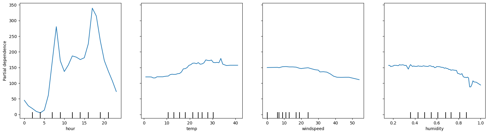
fig, ax = plt.subplots(figsize = (20, 5))
PartialDependenceDisplay.from_estimator(reg, X_test, features = ['hour', 'temp', 'windspeed', 'humidity'],  n_cols = 4,ax = ax)
<sklearn.inspection._plot.partial_dependence.PartialDependenceDisplay at 0x16099b680>
fig, ax = plt.subplots(figsize = (20, 5))
PartialDependenceDisplay.from_estimator(reg, X_test, features = ['hour', 'temp', 'windspeed', 'humidity'],
                                        kind = 'both',
                                        n_cols = 4,ax = ax,
                                       subsample = 30)
<sklearn.inspection._plot.partial_dependence.PartialDependenceDisplay at 0x1775c7200>
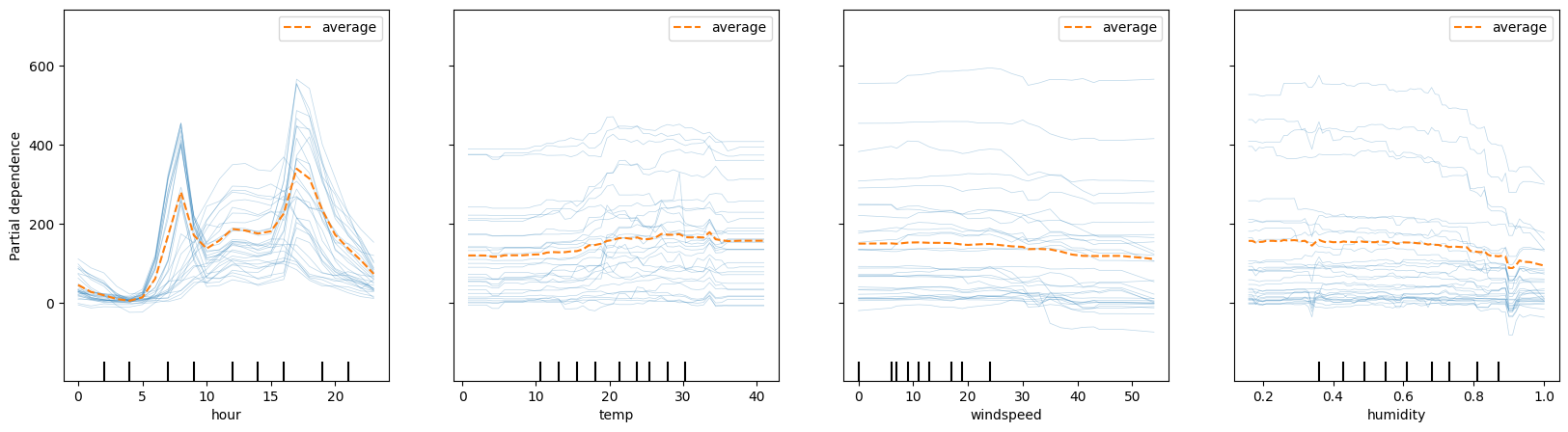
We can also explore two variable PDP plots to understand interactions between features. Note the wiggles in the ICE plots above with temperature and humidity.
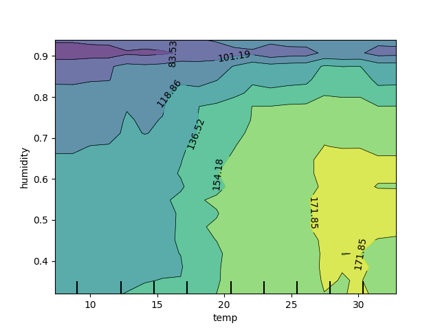
# Slower to plot the 2-way PDP
# PartialDependenceDisplay.from_estimator(reg, X_train, [('temp', 'humidity')], subsample = 50, n_jobs = -1, grid_resolution=20, kind = 'average' )
Permutation Feature Importance
Permute individual features while holding others constant to see the effect on target.
results = permutation_importance(reg, X_train, y_train, n_repeats=10)
results
{'importances_mean': array([0.06408446, 0.        , 0.05608611, 1.38907729, 0.00536676,
        0.03095871, 0.26588249, 0.03003684, 0.09342833, 0.06718443,
        0.09206399, 0.01775954]),
 'importances_std': array([0.00146776, 0.        , 0.00142307, 0.02330278, 0.00026406,
        0.00068182, 0.00639445, 0.00058722, 0.00220706, 0.00162217,
        0.00358808, 0.0007023 ]),
 'importances': array([[0.06300265, 0.06402278, 0.06463879, 0.06582814, 0.06204641,
         0.06684893, 0.06517816, 0.06249613, 0.06286907, 0.06391352],
        [0.        , 0.        , 0.        , 0.        , 0.        ,
         0.        , 0.        , 0.        , 0.        , 0.        ],
        [0.05552417, 0.05325413, 0.05561483, 0.05599797, 0.05715764,
         0.05666196, 0.05552161, 0.05509174, 0.05717289, 0.05886412],
        [1.39215404, 1.38278419, 1.39891392, 1.43035001, 1.39482099,
         1.3678748 , 1.39885134, 1.41269845, 1.36795563, 1.34436959],
        [0.00556594, 0.00533265, 0.00586772, 0.00505203, 0.00564623,
         0.005108  , 0.00524527, 0.00502574, 0.00529748, 0.00552654],
        [0.03143972, 0.03074974, 0.03096807, 0.03105378, 0.03102279,
         0.03210676, 0.03005022, 0.0318892 , 0.02998865, 0.03031814],
        [0.26693612, 0.27388686, 0.26138693, 0.26471162, 0.25932431,
         0.27060401, 0.25526071, 0.27479178, 0.26027721, 0.27164531],
        [0.03051323, 0.02920526, 0.03001463, 0.03068423, 0.02960652,
         0.02993691, 0.03099948, 0.02955091, 0.0305323 , 0.02932495],
        [0.0908969 , 0.09123766, 0.09405136, 0.09543508, 0.09107119,
         0.09412605, 0.09672433, 0.0918116 , 0.09207493, 0.09685421],
        [0.06753367, 0.06542045, 0.06594509, 0.06789696, 0.06580669,
         0.06691229, 0.06712925, 0.06528443, 0.06977129, 0.07014418],
        [0.09755111, 0.0880959 , 0.08526027, 0.08980298, 0.09112072,
         0.09527755, 0.09177947, 0.09575665, 0.09144682, 0.0945484 ],
        [0.01812655, 0.01650363, 0.01809645, 0.01843345, 0.01672405,
         0.01816964, 0.01718265, 0.01865005, 0.01822078, 0.01748812]])}
pd.DataFrame(results['importances'], index = X_train.columns.tolist()).T.plot(kind = 'box', vert = False)
<Axes: >
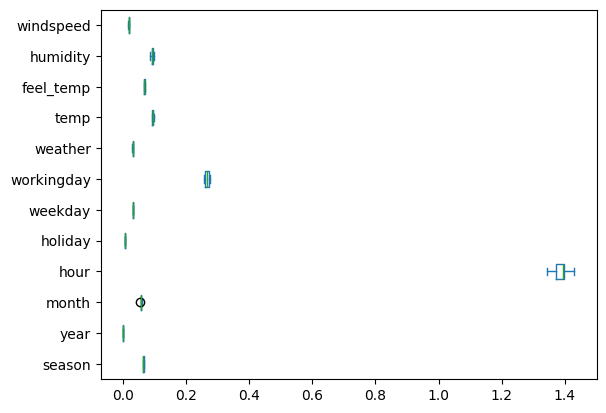
pd.DataFrame(results['importances_mean'], index = X_train.columns.tolist()).sort_values(0, ascending = False)
| 0 | |
|---|---|
| hour | 1.389077 |
| workingday | 0.265882 |
| temp | 0.093428 |
| humidity | 0.092064 |
| feel_temp | 0.067184 |
| season | 0.064084 |
| month | 0.056086 |
| weekday | 0.030959 |
| weather | 0.030037 |
| windspeed | 0.017760 |
| holiday | 0.005367 |
| year | 0.000000 |
Comparing Boosted Models#
Returning to the food marketing data from last class:
Can you tune a boosted model to do better than the baseline and optimize towards precision?
What features were important to making these predictions and how would you suggest targeting future customers?
food_marketing = pd.read_csv('https://raw.githubusercontent.com/jfkoehler/nyu_bootcamp_fa25/refs/heads/main/data/food_data.csv')
food_marketing.head()
| ID | Year_Birth | Education | Marital_Status | Income | Kidhome | Teenhome | Dt_Customer | Recency | MntWines | MntFruits | MntMeatProducts | MntFishProducts | MntSweetProducts | MntGoldProds | NumDealsPurchases | NumWebPurchases | NumCatalogPurchases | NumStorePurchases | NumWebVisitsMonth | AcceptedCmp3 | AcceptedCmp4 | AcceptedCmp5 | AcceptedCmp1 | AcceptedCmp2 | Complain | Z_CostContact | Z_Revenue | Response | |
|---|---|---|---|---|---|---|---|---|---|---|---|---|---|---|---|---|---|---|---|---|---|---|---|---|---|---|---|---|---|
| 0 | 5524 | 1957 | Graduation | Single | 58138.0 | 0 | 0 | 2012-09-04 | 58 | 635 | 88 | 546 | 172 | 88 | 88 | 3 | 8 | 10 | 4 | 7 | 0 | 0 | 0 | 0 | 0 | 0 | 3 | 11 | 1 |
| 1 | 2174 | 1954 | Graduation | Single | 46344.0 | 1 | 1 | 2014-03-08 | 38 | 11 | 1 | 6 | 2 | 1 | 6 | 2 | 1 | 1 | 2 | 5 | 0 | 0 | 0 | 0 | 0 | 0 | 3 | 11 | 0 |
| 2 | 4141 | 1965 | Graduation | Together | 71613.0 | 0 | 0 | 2013-08-21 | 26 | 426 | 49 | 127 | 111 | 21 | 42 | 1 | 8 | 2 | 10 | 4 | 0 | 0 | 0 | 0 | 0 | 0 | 3 | 11 | 0 |
| 3 | 6182 | 1984 | Graduation | Together | 26646.0 | 1 | 0 | 2014-02-10 | 26 | 11 | 4 | 20 | 10 | 3 | 5 | 2 | 2 | 0 | 4 | 6 | 0 | 0 | 0 | 0 | 0 | 0 | 3 | 11 | 0 |
| 4 | 5324 | 1981 | PhD | Married | 58293.0 | 1 | 0 | 2014-01-19 | 94 | 173 | 43 | 118 | 46 | 27 | 15 | 5 | 5 | 3 | 6 | 5 | 0 | 0 | 0 | 0 | 0 | 0 | 3 | 11 | 0 |
food_marketing.info()
<class 'pandas.core.frame.DataFrame'>
RangeIndex: 2240 entries, 0 to 2239
Data columns (total 29 columns):
 #   Column               Non-Null Count  Dtype
---  ------               --------------  -----
 0   ID                   2240 non-null   int64
 1   Year_Birth           2240 non-null   int64
 2   Education            2240 non-null   object
 3   Marital_Status       2240 non-null   object
 4   Income               2216 non-null   float64
 5   Kidhome              2240 non-null   int64
 6   Teenhome             2240 non-null   int64
 7   Dt_Customer          2240 non-null   object
 8   Recency              2240 non-null   int64
 9   MntWines             2240 non-null   int64
 10  MntFruits            2240 non-null   int64
 11  MntMeatProducts      2240 non-null   int64
 12  MntFishProducts      2240 non-null   int64
 13  MntSweetProducts     2240 non-null   int64
 14  MntGoldProds         2240 non-null   int64
 15  NumDealsPurchases    2240 non-null   int64
 16  NumWebPurchases      2240 non-null   int64
 17  NumCatalogPurchases  2240 non-null   int64
 18  NumStorePurchases    2240 non-null   int64
 19  NumWebVisitsMonth    2240 non-null   int64
 20  AcceptedCmp3         2240 non-null   int64
 21  AcceptedCmp4         2240 non-null   int64
 22  AcceptedCmp5         2240 non-null   int64
 23  AcceptedCmp1         2240 non-null   int64
 24  AcceptedCmp2         2240 non-null   int64
 25  Complain             2240 non-null   int64
 26  Z_CostContact        2240 non-null   int64
 27  Z_Revenue            2240 non-null   int64
 28  Response             2240 non-null   int64
dtypes: float64(1), int64(25), object(3)
memory usage: 507.6+ KB
food_marketing[['Education', 'Marital_Status']] = food_marketing[['Education', 'Marital_Status']].astype('category')
food_marketing.drop(columns = 'Dt_Customer', inplace = True)
X = food_marketing.drop(columns = 'Response')
y = food_marketing['Response']
X_train, X_test, y_train, y_test = train_test_split(X, y, stratify=y, random_state=10)
PROBLEM#
Below, a dataset around an email campaign for sales is loaded and displayed. Explore the description of the task here. Consider a strategy for model building and evaluation.
# !pip install scikit-uplift
from sklift.datasets import fetch_hillstrom
dataset = fetch_hillstrom(target_col='conversion')
data, target, treatment = dataset.data, dataset.target, dataset.treatment
data.head()
| recency | history_segment | history | mens | womens | zip_code | newbie | channel | |
|---|---|---|---|---|---|---|---|---|
| 0 | 10 | 2) $100 - $200 | 142.44 | 1 | 0 | Surburban | 0 | Phone |
| 1 | 6 | 3) $200 - $350 | 329.08 | 1 | 1 | Rural | 1 | Web |
| 2 | 7 | 2) $100 - $200 | 180.65 | 0 | 1 | Surburban | 1 | Web |
| 3 | 9 | 5) $500 - $750 | 675.83 | 1 | 0 | Rural | 1 | Web |
| 4 | 2 | 1) $0 - $100 | 45.34 | 1 | 0 | Urban | 0 | Web |
target.head()
0    0
1    0
2    0
3    0
4    0
Name: conversion, dtype: int64
treatment.head()
0    Womens E-Mail
1        No E-Mail
2    Womens E-Mail
3      Mens E-Mail
4    Womens E-Mail
Name: segment, dtype: object