Forecasting with sktime

OBJECTIVES

• Basic forecasting workflow with sktime library

• Exponential Smoothing models

• Holt Winters Model

• Autoregression

• ARIMA Models

Starting from our last notebook, today we will cover additional forecasting models and further use sktime to implement time series forecasting models. We will use data that is already prepared as we discussed – datetime index sorted in time.

Grid Searching a Pipeline

The example below demonstrates gridsearching elements of a pipeline. How does this work?

from sklearn.model_selection import GridSearchCV
from sklearn.preprocessing import OneHotEncoder, PolynomialFeatures
from sklearn.ensemble import RandomForestRegressor
from sklearn.datasets import fetch_openml
from sklearn.compose import make_column_transformer
from sklearn.pipeline import Pipeline
from sklearn import set_config

import pandas as pd
import numpy as np
import matplotlib.pyplot as plt
import warnings
warnings.filterwarnings('ignore')

set_config(transform_output='pandas')

survey = fetch_openml(data_id=534, as_frame=True)

X = survey.data
y = survey.target

X.head()

	EDUCATION	SOUTH	SEX	EXPERIENCE	UNION	AGE	RACE	OCCUPATION	SECTOR	MARR
0	8	no	female	21	not_member	35	Hispanic	Other	Manufacturing	Married
1	9	no	female	42	not_member	57	White	Other	Manufacturing	Married
2	12	no	male	1	not_member	19	White	Other	Manufacturing	Unmarried
3	12	no	male	4	not_member	22	White	Other	Other	Unmarried
4	12	no	male	17	not_member	35	White	Other	Other	Married

cat_cols = X.select_dtypes('category').columns.tolist()

ohe = OneHotEncoder(sparse_output=False, handle_unknown = 'ignore')
transformer = make_column_transformer((ohe, cat_cols), remainder = 'passthrough',
                                     verbose_feature_names_out=False)

forest = RandomForestRegressor()

pipe = Pipeline([('transformer', transformer), ('model', forest)])

#what is happening here?
params = {'model__n_estimators': [10, 100],
          'model__max_depth': [1, 2, 3, None],
          'transformer__remainder': ['passthrough', PolynomialFeatures(interaction_only=True)]}

grid = GridSearchCV(pipe, param_grid=params)

grid.fit(X, y)

GridSearchCV(estimator=Pipeline(steps=[('transformer',
                                        ColumnTransformer(remainder='passthrough',
                                                          transformers=[('onehotencoder',
                                                                         OneHotEncoder(handle_unknown='ignore',
                                                                                       sparse_output=False),
                                                                         ['SOUTH',
                                                                          'SEX',
                                                                          'UNION',
                                                                          'RACE',
                                                                          'OCCUPATION',
                                                                          'SECTOR',
                                                                          'MARR'])],
                                                          verbose_feature_names_out=False)),
                                       ('model', RandomForestRegressor())]),
             param_grid={'model__max_depth': [1, 2, 3, None],
                         'model__n_estimators': [10, 100],
                         'transformer__remainder': ['passthrough',
                                                    PolynomialFeatures(interaction_only=True)]})

In a Jupyter environment, please rerun this cell to show the HTML representation or trust the notebook.
On GitHub, the HTML representation is unable to render, please try loading this page with nbviewer.org.

grid.best_params_

{'model__max_depth': 3,
 'model__n_estimators': 10,
 'transformer__remainder': 'passthrough'}

grid.score(X, y)

0.38913228679664846

Add a search over the max_depth parameter of the RandomForestRegressor where you consider trees with:

max_depth = [1, 2, 3, None]

Feature Importances

The RandomForestRegressor has .feature_importances_ determined by the use of a feature in splitting. Below these are displayed as a DataFrame.

steps = grid.best_estimator_.named_steps

pd.DataFrame(steps['model'].feature_importances_, 
             index = steps['transformer'].get_feature_names_out(),
            columns = ['feature importance'])\
            .sort_values(by = 'feature importance', 
            ascending = False)

	feature importance
EDUCATION	0.342572
AGE	0.182168
OCCUPATION_Management	0.090434
EXPERIENCE	0.083535
UNION_member	0.071556
OCCUPATION_Professional	0.067443
SEX_male	0.046405
OCCUPATION_Service	0.035763
UNION_not_member	0.028049
SECTOR_Manufacturing	0.027035
SOUTH_no	0.016813
RACE_Other	0.005194
OCCUPATION_Clerical	0.003034
SOUTH_yes	0.000000
OCCUPATION_Sales	0.000000
RACE_White	0.000000
SECTOR_Construction	0.000000
SECTOR_Other	0.000000
MARR_Married	0.000000
MARR_Unmarried	0.000000
RACE_Hispanic	0.000000
SEX_female	0.000000
OCCUPATION_Other	0.000000

sktime

#!pip install sktime[all_extras]

import sktime as skt

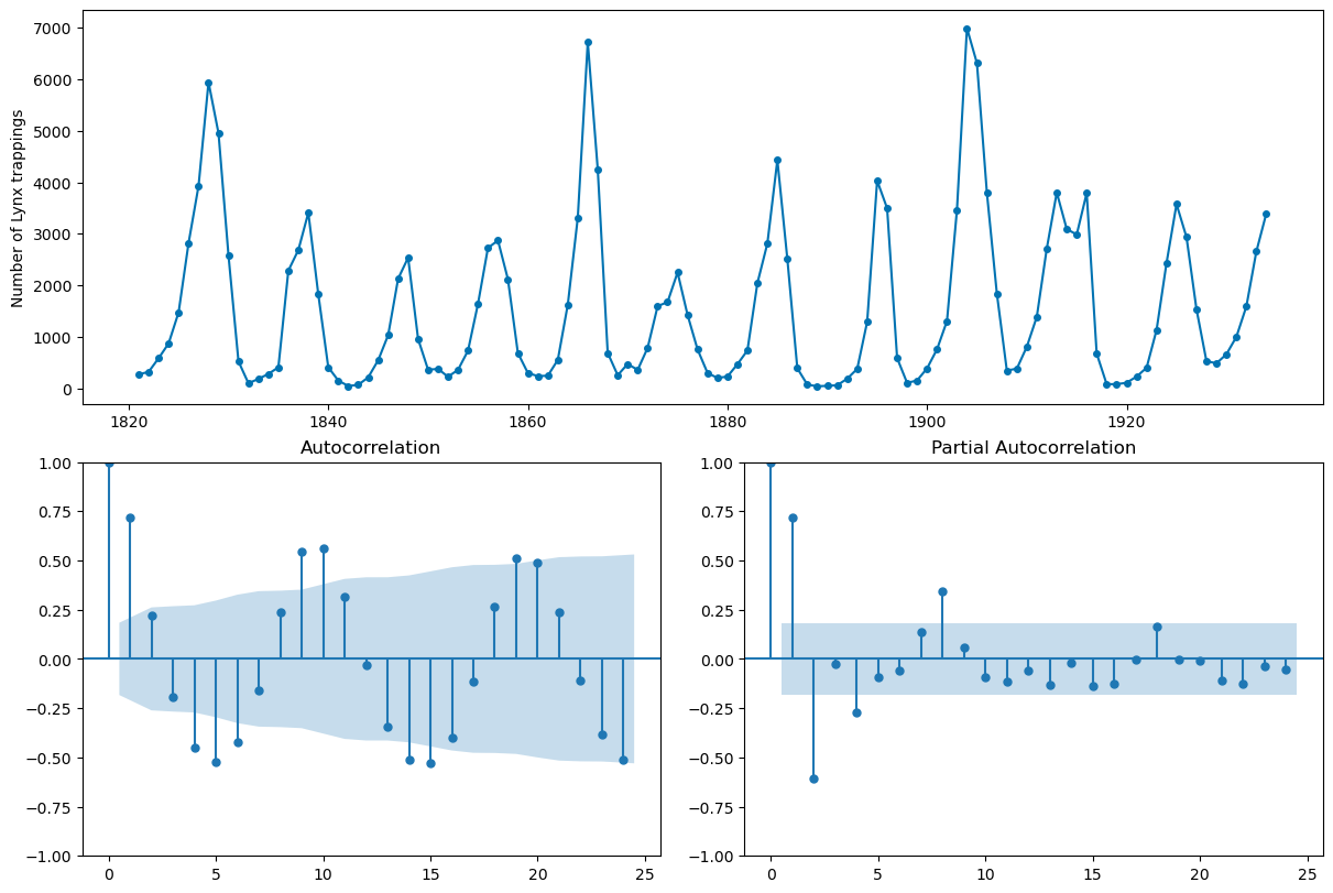
from sktime.datasets import load_lynx
from sktime.utils.plotting import plot_correlations, plot_series

Visualizing Time Series

Initially, it is important to consider a plot of the series. Here, we are looking at the very least to see if the series has a trend or some kind of seasonality. We will typically also look to the autocorrelation and partial autocorrelation plot.

• plot_series

• plot_correlations

lynx = load_lynx()

plot_series(lynx);

---------------------------------------------------------------------------
ImportError                               Traceback (most recent call last)
Cell In[21], line 1
----> 1 plot_series(lynx);

File /Library/Frameworks/Python.framework/Versions/3.12/lib/python3.12/site-packages/sktime/utils/plotting.py:90, in plot_series(labels, markers, colors, title, x_label, y_label, ax, pred_interval, *series)
     87     check_y(y)
     89 l_series = list(series)
---> 90 l_series = [convert_to(y, "pd.Series", "Series") for y in l_series]
     91 for i in range(len(l_series)):
     92     if isinstance(list(series)[i], pd.DataFrame):

File /Library/Frameworks/Python.framework/Versions/3.12/lib/python3.12/site-packages/sktime/datatypes/_convert.py:265, in convert_to(obj, to_type, as_scitype, store, store_behaviour, return_to_mtype)
    262     as_scitype = mtype_to_scitype(to_type)
    264 # now further narrow down as_scitype by inference from the obj
--> 265 from_type = infer_mtype(obj=obj, as_scitype=as_scitype)
    266 as_scitype = mtype_to_scitype(from_type)
    268 converted_obj = convert(
    269     obj=obj,
    270     from_type=from_type,
   (...)
    275     return_to_mtype=return_to_mtype,
    276 )

File /Library/Frameworks/Python.framework/Versions/3.12/lib/python3.12/site-packages/sktime/datatypes/_check.py:359, in mtype(obj, as_scitype, exclude_mtypes)
    357     as_scitype = _coerce_list_of_str(as_scitype, var_name="as_scitype")
    358     for scitype in as_scitype:
--> 359         _check_scitype_valid(scitype)
    361 check_dict = get_check_dict()
    362 m_plus_scitypes = [
    363     (x[0], x[1]) for x in check_dict.keys() if x[0] not in exclude_mtypes
    364 ]

File /Library/Frameworks/Python.framework/Versions/3.12/lib/python3.12/site-packages/sktime/datatypes/_check.py:92, in _check_scitype_valid(scitype)
     90 def _check_scitype_valid(scitype: str = None):
     91     """Check validity of scitype."""
---> 92     check_dict = get_check_dict()
     93     valid_scitypes = list({x[1] for x in check_dict.keys()})
     95     if not isinstance(scitype, str):

File /Library/Frameworks/Python.framework/Versions/3.12/lib/python3.12/site-packages/sktime/datatypes/_check.py:52, in get_check_dict(soft_deps)
     47 if soft_deps not in ["present", "all"]:
     48     raise ValueError(
     49         "Error in get_check_dict, soft_deps argument must be 'present' or 'all', "
     50         f"found {soft_deps}"
     51     )
---> 52 check_dict = generate_check_dict(soft_deps=soft_deps)
     53 return check_dict.copy()

File /Library/Frameworks/Python.framework/Versions/3.12/lib/python3.12/site-packages/sktime/datatypes/_check.py:59, in generate_check_dict(soft_deps)
     56 @lru_cache(maxsize=1)
     57 def generate_check_dict(soft_deps="present"):
     58     """Generate check_dict using lookup."""
---> 59     from skbase.utils.dependencies import _check_estimator_deps
     61     from sktime.utils.retrieval import _all_classes
     63     classes = _all_classes("sktime.datatypes")

ImportError: cannot import name '_check_estimator_deps' from 'skbase.utils.dependencies' (/Library/Frameworks/Python.framework/Versions/3.12/lib/python3.12/site-packages/skbase/utils/dependencies/__init__.py)

plot_correlations(lynx);

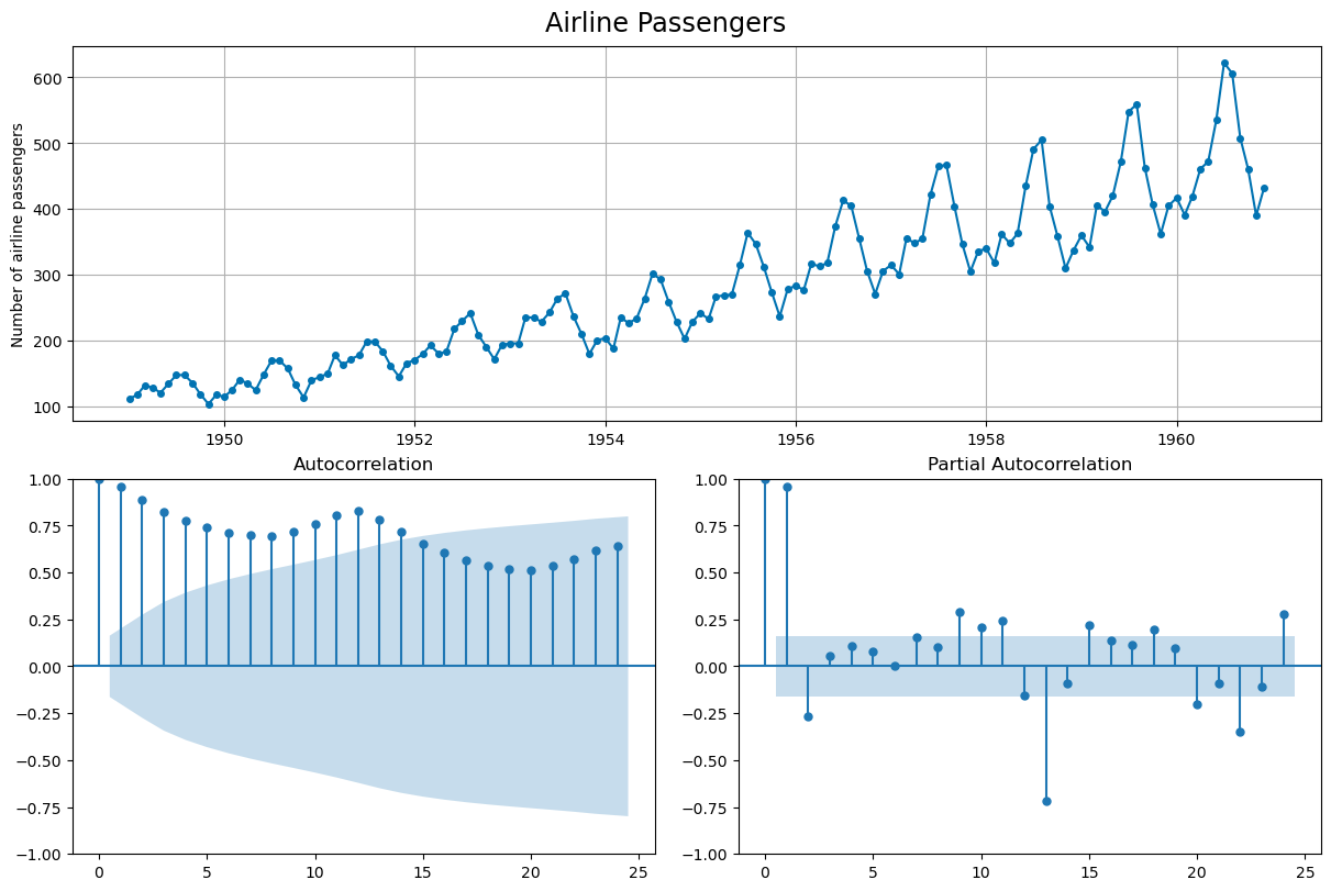
Forecasting with sktime

from sktime.datasets import load_airline

airline = load_airline()

_, ax = plot_correlations(airline, suptitle = 'Airline Passengers')
ax[0].grid()

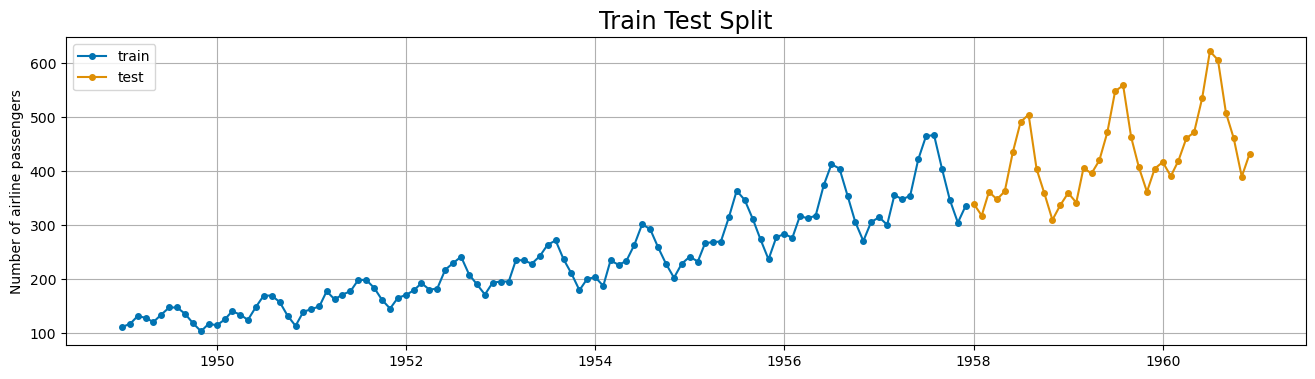
from sktime.split import temporal_train_test_split

X_train, X_test = temporal_train_test_split(airline)

plot_series(X_train, X_test, labels = ['train', 'test'], title = 'Train Test Split')
plt.grid();

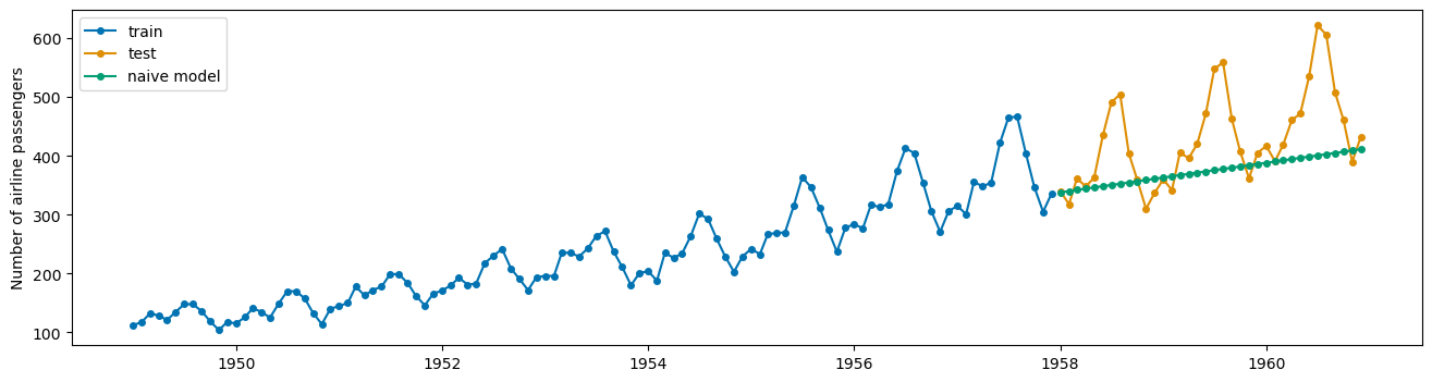
Baseline Model

The NaiveForecaster provides multiple strategies for baseline predicitions. What does stragey = 'drift' do? Plot the predictions along with the train and test data adding appropriate labels.

from sktime.forecasting.naive import NaiveForecaster

#number of time steps to forecast
fh = np.arange(1, len(X_test)+1)
fh

array([ 1,  2,  3,  4,  5,  6,  7,  8,  9, 10, 11, 12, 13, 14, 15, 16, 17,
       18, 19, 20, 21, 22, 23, 24, 25, 26, 27, 28, 29, 30, 31, 32, 33, 34,
       35, 36])

#instantiate
forecaster = NaiveForecaster(strategy = 'drift')
#fit model
forecaster.fit(X_train)
#predict for horizon
yhat = forecaster.predict(fh)

#plot the predictions using plot_series
plot_series(X_train, X_test, yhat, labels = ['train', 'test', 'naive model'])

(<Figure size 1600x400 with 1 Axes>,
 <Axes: ylabel='Number of airline passengers'>)

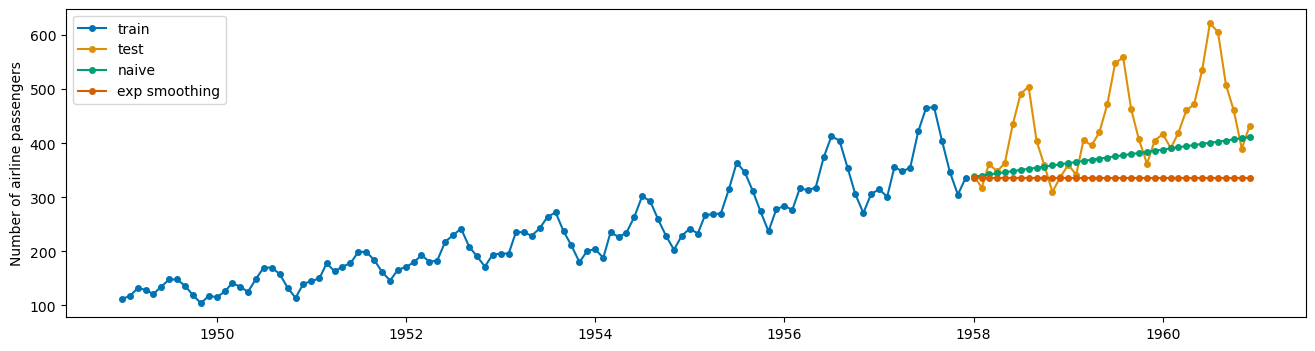
Evaluating predictions

sktime implements many evaluation metrics. Below, the MeanAbsolutePercentageError class is instantiated and used to evaluated the naive baseline. Per usual, lower is better.

from sktime.performance_metrics.forecasting import MeanAbsolutePercentageError

mae = MeanAbsolutePercentageError()

mae(X_test, yhat)

0.1299046419013891

Exponential Smoothing

The weighted moving average model – very basic and simple; predicts the same value over and over.

from sktime.forecasting.exp_smoothing import ExponentialSmoothing

#instantiate
exp = ExponentialSmoothing()

#fit the model
exp.fit(X_train)

ExponentialSmoothing()

Please rerun this cell to show the HTML repr or trust the notebook.

#predict
exp_preds = exp.predict(fh)

#evaluate
mae(X_test, exp_preds)

0.19886712021864697

#plot the series
plot_series(X_train, X_test, yhat, exp_preds, labels = ['train', 'test', 'naive', 'exp smoothing'])

(<Figure size 1600x400 with 1 Axes>,
 <Axes: ylabel='Number of airline passengers'>)

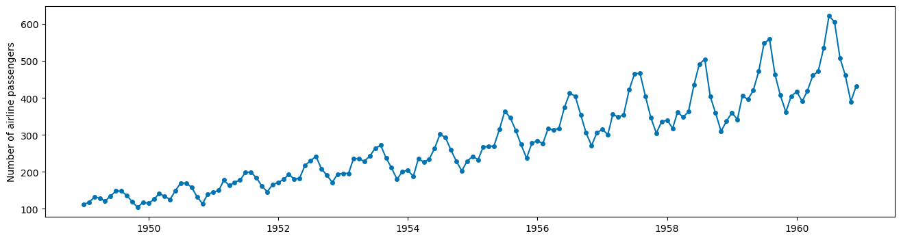
Holt Winters Model

Triple Exponential Smoothing where trend and seasonality are considered. Below, a holt winters model is implemented.

• trend: always additive

• seasonality: additive if same each season, multiplicative if growing

• sp: timesteps in a season

QUESTION: What kind of seasonality should we use here – additive or multiplicative? Why?

#what kind of seasonality?
plot_series(airline);

hw = ExponentialSmoothing(trend = 'add', seasonal='mul', sp = 12)
hw.fit(X_train)
hw_preds = hw.predict(fh)
plot_series(X_train, X_test, hw_preds, 
            labels = ['train', 'test', 'holt winters'],
           )
plt.grid();

mae(X_test, hw_preds)

0.05056484561299068

Stationarity and Differencing

Regression models in time series will also have assumptions about the data, namely that the data we model is stationary. Stationary data has constant mean and variance – thus trends and seasonality are not a part of stationary time series.

plot_correlations(X_train);

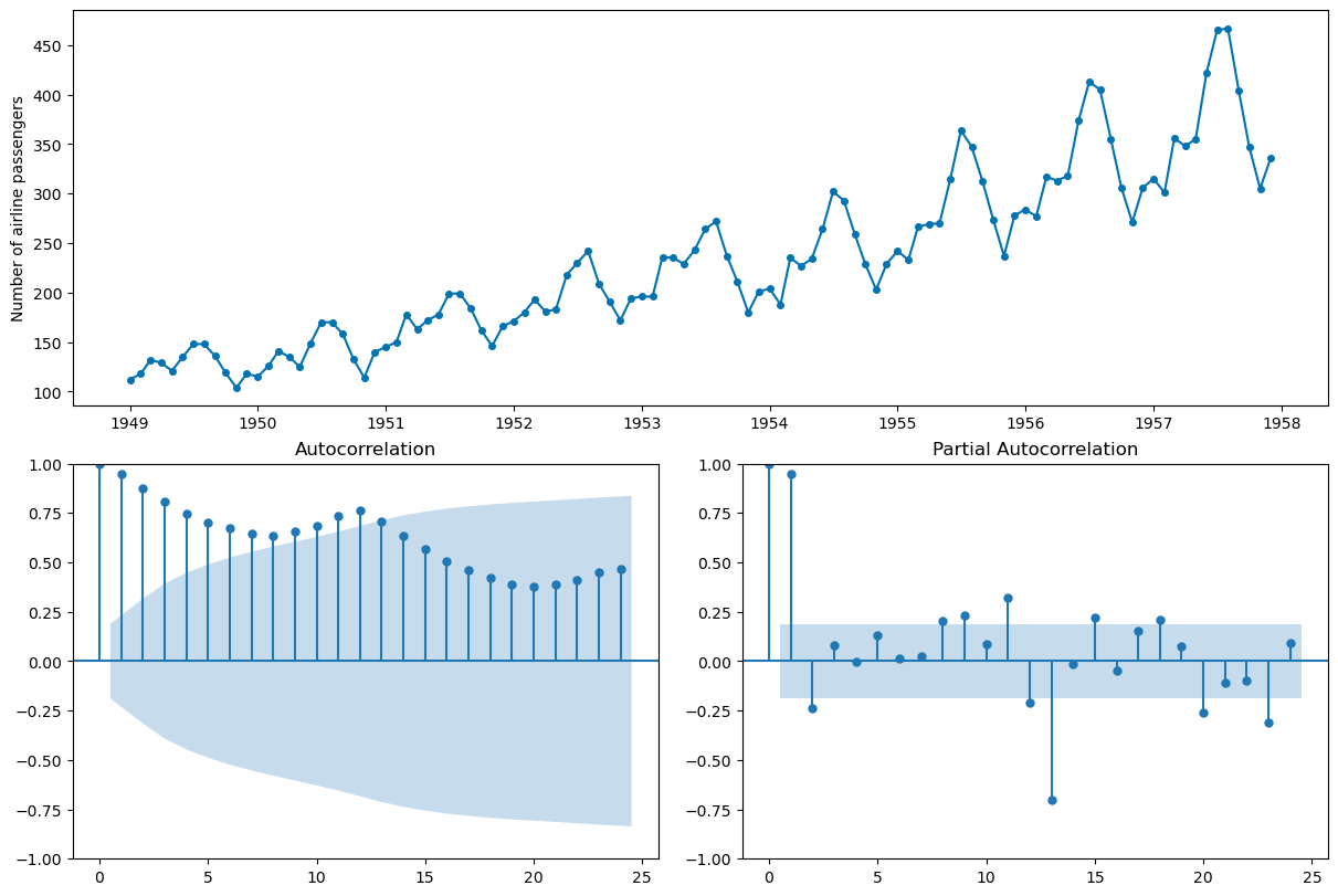
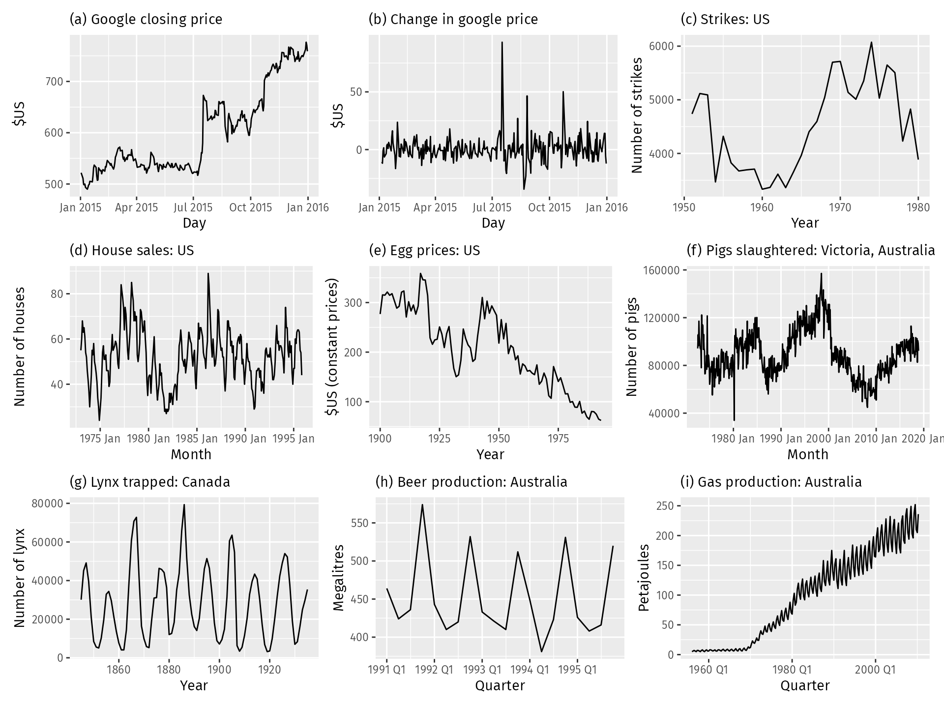
QUESTION: Which of the time series pictured below are stationary?

Differencing the Data

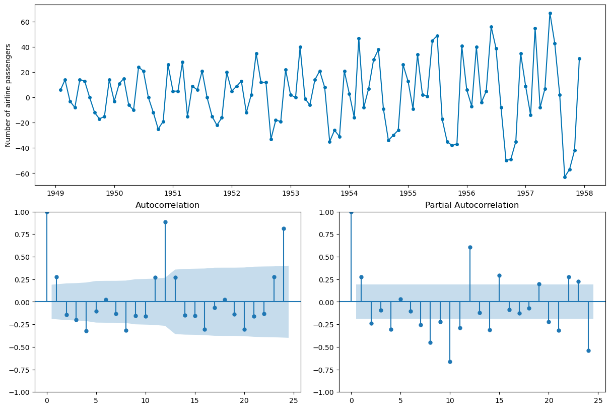
One way to remove the trend is to difference the data. Compare the resulting autocorrelation plot to the undifferenced data.

X_train.diff(1).head()

1949-01     NaN
1949-02     6.0
1949-03    14.0
1949-04    -3.0
1949-05    -8.0
Freq: M, Name: Number of airline passengers, dtype: float64

plot_correlations(X_train.diff(1).dropna());

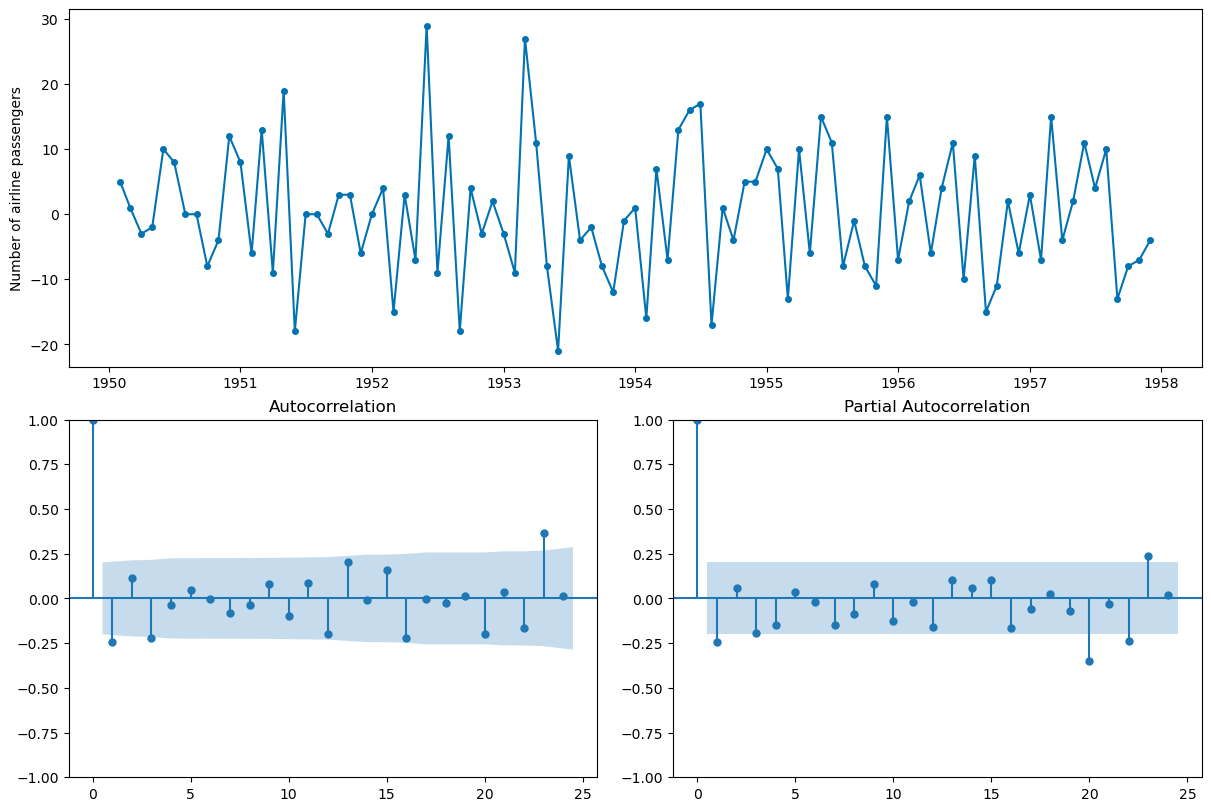
#seasonal differencing to try to remove seasonality -- t and t-12
plot_correlations(X_train.diff(1).diff(12).dropna());

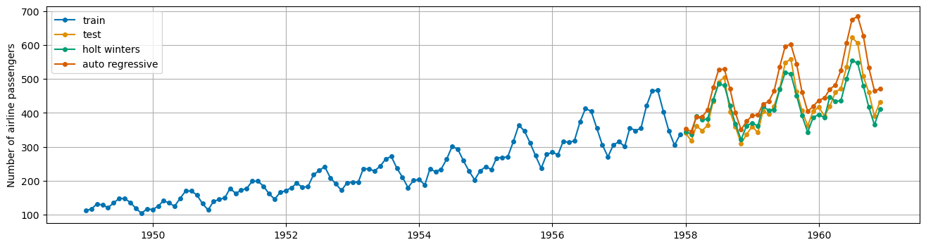
AutoRegression

Similar to regression however the regression is on previous time steps or “lags”.

\[AR(p) = c + \theta_1 y_{t - 1} + \theta_2 y_{t - 2} + ... + \theta_n y_{t - p} + \epsilon\]

from sktime.forecasting.auto_reg import AutoREG

ar = AutoREG(lags = 12)
ar.fit(X_train)
ar_preds = ar.predict(fh)
plot_series(X_train, X_test, hw_preds, ar_preds,
            labels = ['train', 'test', 'holt winters', 'auto regressive'],
           )
plt.grid();

ar.get_fitted_params()

{'aic': 757.542243633855,
 'aicc': 762.7274288190403,
 'bic': 793.4431183144047,
 'hqic': 772.0539637923447,
 'const': 2.9873776849433797,
 'Number of airline passengers.L1': 0.44024802821861964,
 'Number of airline passengers.L2': -0.24712930495045438,
 'Number of airline passengers.L3': 0.19596577672853754,
 'Number of airline passengers.L4': -0.23300070381218363,
 'Number of airline passengers.L5': 0.2307885835405692,
 'Number of airline passengers.L6': -0.17243176175515784,
 'Number of airline passengers.L7': 0.14303113614100504,
 'Number of airline passengers.L8': -0.22605487868090735,
 'Number of airline passengers.L9': 0.22902051756885133,
 'Number of airline passengers.L10': -0.2242183998876448,
 'Number of airline passengers.L11': 0.3190313152823776,
 'Number of airline passengers.L12': 0.6340912733182218}

mae(X_test, ar_preds)

0.10913989054790951

PROBLEM: Adjusting for lags. Consider an autoregressive model that uses the 12 previous time steps to forecast. Is this model better? Plot the results.

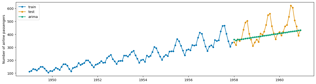
ARIMA models

• AR: Autoregressive component as above

• MA: Moving average of errors

\[MA(q) = c + \epsilon_t + \theta_1 \epsilon_{t+1} + ... + \theta_q \epsilon_{t - q}\]

• ARIMA: Autoregressive integrated moving average

\[ARIMA(p, q, d) = c + \phi_1 y_{t-1} + \phi_2 y_{t-2} + ... + \phi_p y_{t - p} + \theta_1 \epsilon_{t-1} + ... + \epsilon_{t - q} + \epsilon_t\]

• \(p\): order of autoregressive component

• \(q\): order of moving average component

• \(d\): order of differences of series

from sktime.forecasting.arima import ARIMA

arima = ARIMA(order = (1, 1, 1))

arima.fit(X_train)

ARIMA(order=(1, 1, 1))

Please rerun this cell to show the HTML repr or trust the notebook.

arima_preds = arima.predict(fh)

plot_series(X_train, X_test, arima_preds, labels = ['train', 'test', 'arima'])

(<Figure size 1600x400 with 1 Axes>,
 <Axes: ylabel='Number of airline passengers'>)

PROBLEM

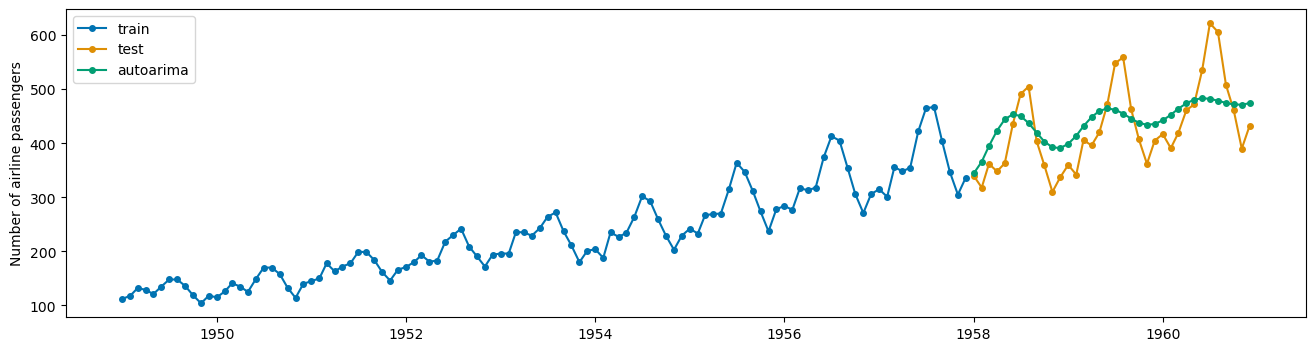
Try to fit an AutoARIMA model (automatically selects \(p,q,d\)). How does this model perform?

from sktime.forecasting.arima import AutoARIMA

#instantiate
auto_ar = AutoARIMA()
#fit
auto_ar.fit(X_train)
#predict
auto_preds = auto_ar.predict(fh)
#print mape
print(mae(X_test, auto_preds))
#plot predictions
plot_series(X_train, X_test, auto_preds, labels = ['train', 'test', 'autoarima'])

0.11654169318875225

(<Figure size 1600x400 with 1 Axes>,
 <Axes: ylabel='Number of airline passengers'>)

auto_ar.get_fitted_params()

{'intercept': 0.6708145063428641,
 'ar.L1': 1.640537387976563,
 'ar.L2': -0.9086368984722021,
 'ma.L1': -1.8337763227623853,
 'ma.L2': 0.9289381223972486,
 'sigma2': 393.3177514621617,
 'order': (2, 1, 2),
 'seasonal_order': (0, 0, 0, 0),
 'aic': 959.2179634640711,
 'aicc': 960.0579634640711,
 'bic': 975.2549364708425,
 'hqic': 965.7191390772085}

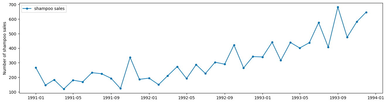
Example: Shampoo Sales

from sktime.datasets import load_shampoo_sales

shampoo = load_shampoo_sales()
plot_series(shampoo, labels = ['shampoo sales']);

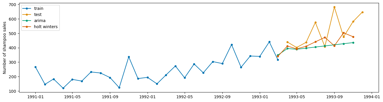
PROBLEM

Split the data into train and test sets to build a Holt Winters model and AutoARIMA model. Compare performance on the test data and plot the resulting predictions using plot_series with appropriate labels.

X_train, X_test = temporal_train_test_split(shampoo)
fh = np.arange(len(X_test))

hw = ExponentialSmoothing(trend = 'add', seasonal='mul', sp = 6)

hw.fit(X_train)

ExponentialSmoothing(seasonal='mul', sp=6, trend='add')

Please rerun this cell to show the HTML repr or trust the notebook.

hw_preds = hw.predict(fh)

auto = AutoARIMA()
auto.fit(X_train)
auto_preds = auto.predict(fh)

plot_series(X_train, X_test, auto_preds, hw_preds, labels = ['train', 'test', 'arima', 'holt winters'])

(<Figure size 1600x400 with 1 Axes>, <Axes: ylabel='Number of shampoo sales'>)

Readings or Watchings:

• Chapter 8.1 - 8.4 of Hyndman here

• Chapter 9 of Hyndman on ARIMA models here