Intro ANN#
Review
numpyandpytorchPerceptron with
numpyandpytorchTraining a basic network with
pytorch
import numpy as np
import matplotlib.pyplot as plt
import torch
from tqdm import tqdm
---------------------------------------------------------------------------
ModuleNotFoundError                       Traceback (most recent call last)
Cell In[1], line 3
      1 import numpy as np
      2 import matplotlib.pyplot as plt
----> 3 import torch
      4 from tqdm import tqdm

ModuleNotFoundError: No module named 'torch'
Derivatives and Gradients for Optimization#
Consider:
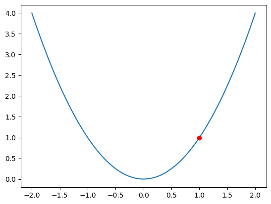
The big idea is that we can use the tangent line at a point to approximate the function itself. Thus, we walk on the tangent line in the negative direction of the slope. If we take small enough steps and readjust each iteration we should find ourselves at the bottom of the graph.
Start at the point \((1, 1)\) and note that the slope of the tangent line is \(f'(1) = 2*1 = 2\).
def f(x): return x**2
x = np.linspace(-2, 2, 100)
plt.plot(x, f(x))
plt.plot(1, 1, 'ro')
[<matplotlib.lines.Line2D at 0x7ce687367880>]
#start - step * slope
1 - .1*(2*1)
0.8
#next step
.8 - .1*(2*.8)
0.64
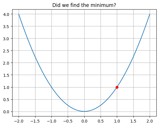
PROBLEM
Complete the loop below, updating the list xs with each iteration of gradient descent.
xs = [1]
for i in range(10):
  pass
xs = np.array(xs)
plt.plot(x, f(x))
plt.plot(xs, f(xs), 'ro')
plt.title('Did we find the minimum?')
plt.grid();
Introduction to Artificial Neural Networks#
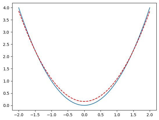
For the examples in our class, we will use the pytorch library for modeling with neural networks. The important object here is the tensor object, similar to the numpy.array but with some extra gradient functionality.
import torch
import torch.nn as nn
import torch.optim as optim
xt = torch.tensor(x, dtype = torch.float32)
yt = torch.tensor(f(x), dtype = torch.float32)
loss_fn = nn.MSELoss()
def model(x, w, b):
  return w*x**2 + b
w = torch.ones((), requires_grad=True)
b = torch.ones((), requires_grad=True)
model(xt, w, b)
tensor([5.0000, 4.8400, 4.6833, 4.5298, 4.3797, 4.2327, 4.0891, 3.9487, 3.8115,
        3.6777, 3.5471, 3.4198, 3.2957, 3.1749, 3.0573, 2.9431, 2.8321, 2.7243,
        2.6198, 2.5186, 2.4207, 2.3260, 2.2346, 2.1464, 2.0615, 1.9799, 1.9015,
        1.8264, 1.7546, 1.6861, 1.6208, 1.5587, 1.4999, 1.4444, 1.3922, 1.3432,
        1.2975, 1.2551, 1.2159, 1.1800, 1.1473, 1.1179, 1.0918, 1.0690, 1.0494,
        1.0331, 1.0200, 1.0102, 1.0037, 1.0004, 1.0004, 1.0037, 1.0102, 1.0200,
        1.0331, 1.0494, 1.0690, 1.0918, 1.1179, 1.1473, 1.1800, 1.2159, 1.2551,
        1.2975, 1.3432, 1.3922, 1.4444, 1.4999, 1.5587, 1.6208, 1.6861, 1.7546,
        1.8264, 1.9015, 1.9799, 2.0615, 2.1464, 2.2346, 2.3260, 2.4207, 2.5186,
        2.6198, 2.7243, 2.8321, 2.9431, 3.0573, 3.1749, 3.2957, 3.4198, 3.5471,
        3.6777, 3.8115, 3.9487, 4.0891, 4.2327, 4.3797, 4.5298, 4.6833, 4.8400,
        5.0000], grad_fn=<AddBackward0>)
yhat = model(xt, w, b)
loss = loss_fn(yt, yhat)
loss.backward()
w.grad
tensor(2.7205)
b.grad
tensor(2.)
#loss.zero_()
optimizer = optim.SGD([w, b], lr = 0.1)
for epoch in tqdm(range(20)):
  yhat = model(xt, w, b)
  loss = loss_fn(yt, yhat)
  loss.backward()
  optimizer.step()
  optimizer.zero_grad()
100%|██████████| 20/20 [00:00<00:00, 2071.62it/s]
w
tensor(0.9263, requires_grad=True)
b
tensor(0.1602, requires_grad=True)
def soln(x): return w.detach().numpy()*x**2 + b.detach().numpy()
plt.plot(x, f(x))
plt.plot(x, soln(x), '--r')
[<matplotlib.lines.Line2D at 0x7ce6874dfd00>]
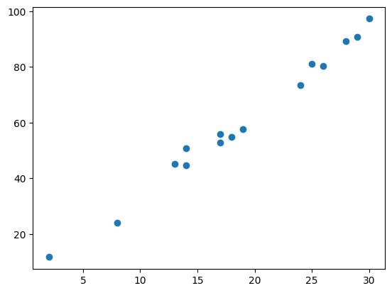
Pytorch and Regression#
np.random.seed(11)
x = np.random.random_integers(low = 1, high = 30, size = 15)
y = 3*x + 4 + np.random.normal(size = len(x), scale = 3)
<ipython-input-616-75502d753c78>:2: DeprecationWarning: This function is deprecated. Please call randint(1, 30 + 1) instead
  x = np.random.random_integers(low = 1, high = 30, size = 15)
plt.scatter(x, y)
<matplotlib.collections.PathCollection at 0x7ce685bd5150>
#rule 1 -- turn everything into a tensor
xt = torch.tensor(x, dtype = torch.float32)
yt = torch.tensor(y, dtype = torch.float32)
xt
tensor([26., 17., 28., 18., 24., 14., 13.,  2.,  8., 19., 25., 14., 29., 17.,
        30.])
yt
tensor([80.3901, 55.9462, 89.2632, 54.8032, 73.3413, 44.5728, 45.0690, 11.6836,
        24.0834, 57.6416, 81.2105, 50.7239, 90.9068, 52.9497, 97.2869])
### define the model
model = nn.Linear(in_features=1, out_features=1)
list(model.parameters())
[Parameter containing:
 tensor([[-0.2880]], requires_grad=True),
 Parameter containing:
 tensor([-0.1145], requires_grad=True)]
loss_fn = nn.MSELoss()
optimizer = optim.SGD(model.parameters(), lr = 0.01)
model(xt.reshape(-1, 1))
tensor([[-7.6035],
        [-5.0112],
        [-8.1796],
        [-5.2992],
        [-7.0275],
        [-4.1471],
        [-3.8590],
        [-0.6906],
        [-2.4188],
        [-5.5873],
        [-7.3155],
        [-4.1471],
        [-8.4676],
        [-5.0112],
        [-8.7557]], grad_fn=<AddmmBackward0>)
yhat = model(xt.reshape(-1, 1))
loss_fn(yt.reshape(-1, 1), yhat )
tensor(5064.9062, grad_fn=<MseLossBackward0>)
loss = loss_fn(yhat, yt.reshape(-1, 1))
loss.backward()
optimizer.step()
list(model.parameters())
[Parameter containing:
 tensor([[28.8443]], requires_grad=True),
 Parameter containing:
 tensor([1.2100], requires_grad=True)]
model = nn.Linear(in_features=1, out_features=1)
loss_fn = nn.MSELoss()
optimizer = optim.Adam(model.parameters(), lr = 0.1)

losses = []
for epoch in tqdm(range(100)):
  yhat = model(xt.reshape(-1, 1))
  loss = loss_fn( yhat, yt.reshape(-1, 1))
  optimizer.zero_grad()
  loss.backward()
  optimizer.step()
  losses.append(loss.item())
100%|██████████| 100/100 [00:00<00:00, 1651.63it/s]
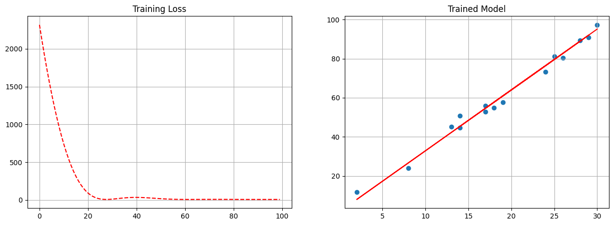
fig, ax = plt.subplots(1, 2, figsize = (15, 5))
ax[0].plot(losses, '--r')
ax[0].set_title('Training Loss')
ax[0].grid();

ax[1].scatter(x, y)
ax[1].plot(x, model(xt.reshape(-1, 1)).detach().numpy(), '-r')
ax[1].set_title('Trained Model')
ax[1].grid();
import pandas as pd
Binary Classification#
Same process but we add a Sigmoid to the end of the network to interpret the output as probabilities.
Loss will use BCELoss or Binary Cross Entropy – a measure associated with the quality of predictions in binary classification.
from sklearn.datasets import make_blobs
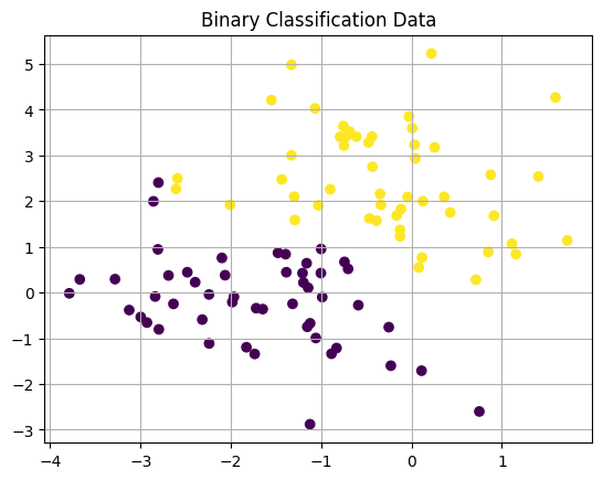
### make a basic classification dataset
X, y = make_blobs(centers = 2, center_box=(-3, 3), random_state = 22)
X.shape
(100, 2)
plt.scatter(X[:, 0], X[:, 1], c = y)
plt.grid()
plt.title('Binary Classification Data');
model = nn.Sequential(nn.Linear(in_features=2, out_features=1), nn.Sigmoid())
# WE NEED BINARY CLASSIFICATION LOSS
loss = nn.BCELoss()
optimizer = optim.SGD(model.parameters(), lr = 0.1)
X = torch.tensor(X, dtype = torch.float32)
y = torch.tensor(y, dtype = torch.float32)
losses = []
for epoch in tqdm(range(100)):
  #make some predictions
  yhat = model(X)
  #evaluate the predictions
  loss_val = loss(yhat, y.unsqueeze(1))
  #use those predictions to update the parameters
  optimizer.zero_grad() #clearing out any prior gradient info
  loss_val.backward() #computes derivatives/gradients of loss function
  optimizer.step() #steps towards minimum values
  #keep track of how we are doing
  losses.append(loss_val.item())
100%|██████████| 100/100 [00:00<00:00, 2096.67it/s]
yhat.dtype
torch.float32
#the model returns probabilities
model(X)[:10]
tensor([[0.7954],
        [0.0077],
        [0.0995],
        [0.0091],
        [0.0183],
        [0.8861],
        [0.9653],
        [0.0081],
        [0.1589],
        [0.9119]], grad_fn=<SliceBackward0>)
torch.where(model(X) > 0.5, 1, 0).flatten()
tensor([1, 0, 0, 0, 0, 1, 1, 0, 0, 1, 0, 0, 1, 0, 0, 1, 1, 1, 1, 1, 1, 0, 1, 0,
        0, 1, 0, 0, 0, 1, 1, 1, 0, 0, 1, 0, 1, 1, 0, 0, 0, 0, 1, 1, 0, 0, 1, 1,
        1, 1, 0, 1, 0, 0, 1, 0, 1, 1, 1, 0, 1, 0, 1, 1, 0, 0, 1, 0, 1, 0, 0, 0,
        1, 0, 0, 1, 0, 0, 1, 1, 1, 1, 1, 1, 1, 0, 0, 1, 0, 0, 1, 1, 1, 1, 0, 0,
        1, 1, 0, 0])
y
tensor([1., 0., 0., 0., 0., 1., 1., 0., 0., 1., 0., 0., 1., 0., 0., 1., 1., 1.,
        1., 1., 1., 0., 1., 0., 0., 1., 0., 0., 0., 1., 1., 1., 0., 0., 1., 0.,
        1., 1., 0., 0., 0., 0., 1., 1., 0., 0., 1., 1., 1., 1., 0., 1., 0., 0.,
        1., 0., 1., 1., 1., 0., 1., 0., 0., 1., 0., 0., 1., 0., 1., 0., 0., 0.,
        1., 0., 0., 1., 0., 0., 1., 1., 1., 1., 1., 1., 1., 0., 0., 1., 0., 0.,
        1., 1., 1., 1., 0., 0., 1., 1., 0., 0.])
torch.where(model(X) > 0.5, 1, 0).flatten() == y
tensor([ True,  True,  True,  True,  True,  True,  True,  True,  True,  True,
         True,  True,  True,  True,  True,  True,  True,  True,  True,  True,
         True,  True,  True,  True,  True,  True,  True,  True,  True,  True,
         True,  True,  True,  True,  True,  True,  True,  True,  True,  True,
         True,  True,  True,  True,  True,  True,  True,  True,  True,  True,
         True,  True,  True,  True,  True,  True,  True,  True,  True,  True,
         True,  True, False,  True,  True,  True,  True,  True,  True,  True,
         True,  True,  True,  True,  True,  True,  True,  True,  True,  True,
         True,  True,  True,  True,  True,  True,  True,  True,  True,  True,
         True,  True,  True,  True,  True,  True,  True,  True,  True,  True])
(torch.where(model(X) > 0.5, 1, 0).flatten() == y).sum()
tensor(99)
X.shape
torch.Size([100, 2])
yhat = torch.where(model(X) > 0, 1, 0)
yhat.shape
torch.Size([100, 1])
y == yhat.flatten()
tensor([ True, False, False, False, False,  True,  True, False, False,  True,
        False, False,  True, False, False,  True,  True,  True,  True,  True,
         True, False,  True, False, False,  True, False, False, False,  True,
         True,  True, False, False,  True, False,  True,  True, False, False,
        False, False,  True,  True, False, False,  True,  True,  True,  True,
        False,  True, False, False,  True, False,  True,  True,  True, False,
         True, False, False,  True, False, False,  True, False,  True, False,
        False, False,  True, False, False,  True, False, False,  True,  True,
         True,  True,  True,  True,  True, False, False,  True, False, False,
         True,  True,  True,  True, False, False,  True,  True, False, False])
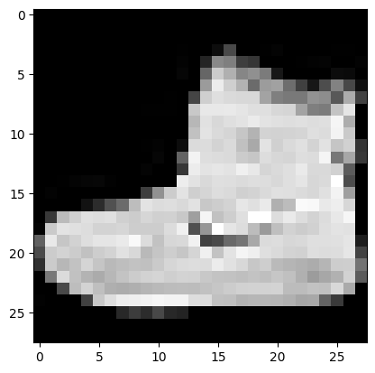
Image Classification#
from torchvision.datasets import FashionMNIST
from torch.utils.data import DataLoader
from torchvision.transforms import ToTensor
train = FashionMNIST(root = './data', train = True, download = True, transform = ToTensor())
test = FashionMNIST(root = './data', train = False, download = True, transform=ToTensor())
trainloader = DataLoader(train, batch_size = 10, shuffle = True)
testloader = DataLoader(test, batch_size = 10, shuffle = False)
plt.imshow(train[0][0].squeeze(0), cmap = 'gray')
<matplotlib.image.AxesImage at 0x7ce685789810>
device = torch.device('cuda' if torch.cuda.is_available() else 'cpu')
model = nn.Sequential(nn.Flatten(),
                      nn.Linear(in_features=28*28, out_features=10))
model = model.to(device)
loss_fn = nn.CrossEntropyLoss()
optimizer = optim.SGD(model.parameters(), lr = 0.1)
device
device(type='cuda')
for epoch in tqdm(range(10)):
  for x, y in trainloader:
    x = x.to(device)
    y = y.to(device)
    yhat = model(x)
    loss = loss_fn(yhat, y)
    optimizer.zero_grad()
    loss.backward()
    optimizer.step()
100%|██████████| 10/10 [02:11<00:00, 13.19s/it]
model(x).argmax(dim = 1)
tensor([7, 5, 4, 4, 3, 4, 8, 3, 7, 4], device='cuda:0')
y
tensor([7, 5, 4, 4, 3, 4, 8, 3, 7, 4], device='cuda:0')
(model(x).argmax(dim = 1) == y).sum()
tensor(10, device='cuda:0')
correct = 0
total = 0
for x, y in testloader:
    x = x.to(device)
    y = y.to(device)
    yhat = model(x)
    correct += (yhat.argmax(dim = 1) == y).sum()
    total += len(y)
print(f'Accuracy: {correct/total}')
Accuracy: 0.8136999607086182