Grid Searching and Time Series Forecasting#
Use the data below to set up a Pipeline that one hot encodes all categorical features and builds a RandomForestClassifier model. Grid search the model for an appropriate n_estimators and max_depth parameter optimizing precision. What were the parameters of the best model?
import pandas as pd
import numpy as np
import matplotlib.pyplot as plt
import seaborn as sns
import warnings
warnings.filterwarnings('ignore')
from sklearn.datasets import fetch_openml
insurance = fetch_openml(data_id=45064)
insurance.frame.head()
| Upper_Age | Lower_Age | Reco_Policy_Premium | City_Code | Accomodation_Type | Reco_Insurance_Type | Is_Spouse | Health Indicator | Holding_Policy_Duration | Holding_Policy_Type | class | |
|---|---|---|---|---|---|---|---|---|---|---|---|
| 0 | 52 | 52 | 16200.0 | C2 | Owned | Individual | No | X4 | 6.0 | 4.0 | 0 |
| 1 | 67 | 67 | 16900.0 | C17 | Rented | Individual | No | X1 | 7.0 | 3.0 | 1 |
| 2 | 75 | 75 | 25668.0 | C10 | Owned | Individual | No | X3 | 3.0 | 1.0 | 0 |
| 3 | 60 | 57 | 17586.8 | C26 | Owned | Joint | Yes | X1 | 14+ | 1.0 | 0 |
| 4 | 35 | 35 | 12762.0 | C12 | Rented | Individual | No | X1 | 3.0 | 2.0 | 0 |
insurance.frame.info()
<class 'pandas.core.frame.DataFrame'>
RangeIndex: 23548 entries, 0 to 23547
Data columns (total 11 columns):
 #   Column                   Non-Null Count  Dtype
---  ------                   --------------  -----
 0   Upper_Age                23548 non-null  int64
 1   Lower_Age                23548 non-null  int64
 2   Reco_Policy_Premium      23548 non-null  float64
 3   City_Code                23548 non-null  category
 4   Accomodation_Type        23548 non-null  category
 5   Reco_Insurance_Type      23548 non-null  category
 6   Is_Spouse                23548 non-null  category
 7   Health Indicator         23548 non-null  category
 8   Holding_Policy_Duration  23548 non-null  category
 9   Holding_Policy_Type      23548 non-null  category
 10  class                    23548 non-null  int64
dtypes: category(7), float64(1), int64(3)
memory usage: 899.9 KB
insurance.frame.describe()
| Upper_Age | Lower_Age | Reco_Policy_Premium | class | |
|---|---|---|---|---|
| count | 23548.000000 | 23548.000000 | 23548.000000 | 23548.000000 |
| mean | 48.864192 | 46.365381 | 15409.000161 | 0.242059 |
| std | 16.021466 | 16.578403 | 6416.327319 | 0.428339 |
| min | 21.000000 | 16.000000 | 3216.000000 | 0.000000 |
| 25% | 35.000000 | 32.000000 | 10704.000000 | 0.000000 |
| 50% | 49.000000 | 46.000000 | 14580.000000 | 0.000000 |
| 75% | 62.000000 | 60.000000 | 19140.000000 | 0.000000 |
| max | 75.000000 | 75.000000 | 43350.400000 | 1.000000 |
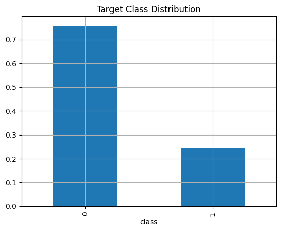
insurance.frame['class'].value_counts(normalize = True).plot(kind = 'bar', grid = True, title = 'Target Class Distribution');
from sklearn.ensemble import RandomForestClassifier
from sklearn.model_selection import train_test_split, GridSearchCV
from sklearn.preprocessing import StandardScaler, OneHotEncoder
from sklearn.metrics import ConfusionMatrixDisplay
from sklearn.pipeline import Pipeline
from sklearn.compose import make_column_transformer
Time Series#
For these problems I will reference Hyndman’s Forecasting: Principles and Practice. At a minimum, skim chapter 8.1 - 8.4 on Exponential Smoothing methods and 9.1 - 9.5 and 9.9 on ARIMA models. We will replicate some examples and problems from the text using sktime. Reference the documentation here when needed.
!pip install sktime
Requirement already satisfied: sktime in /Library/Frameworks/Python.framework/Versions/3.12/lib/python3.12/site-packages (0.34.0)
Requirement already satisfied: joblib<1.5,>=1.2.0 in /Library/Frameworks/Python.framework/Versions/3.12/lib/python3.12/site-packages (from sktime) (1.3.2)
Requirement already satisfied: numpy<2.2,>=1.21 in /Library/Frameworks/Python.framework/Versions/3.12/lib/python3.12/site-packages (from sktime) (1.26.4)
Requirement already satisfied: packaging in /Library/Frameworks/Python.framework/Versions/3.12/lib/python3.12/site-packages (from sktime) (23.2)
Requirement already satisfied: pandas<2.3.0,>=1.1 in /Library/Frameworks/Python.framework/Versions/3.12/lib/python3.12/site-packages (from sktime) (2.2.3)
Requirement already satisfied: scikit-base<0.12.0,>=0.6.1 in /Library/Frameworks/Python.framework/Versions/3.12/lib/python3.12/site-packages (from sktime) (0.6.1)
Requirement already satisfied: scikit-learn<1.6.0,>=0.24 in /Library/Frameworks/Python.framework/Versions/3.12/lib/python3.12/site-packages (from sktime) (1.5.2)
Requirement already satisfied: scipy<2.0.0,>=1.2 in /Library/Frameworks/Python.framework/Versions/3.12/lib/python3.12/site-packages (from sktime) (1.11.4)
Requirement already satisfied: python-dateutil>=2.8.2 in /Library/Frameworks/Python.framework/Versions/3.12/lib/python3.12/site-packages (from pandas<2.3.0,>=1.1->sktime) (2.8.2)
Requirement already satisfied: pytz>=2020.1 in /Library/Frameworks/Python.framework/Versions/3.12/lib/python3.12/site-packages (from pandas<2.3.0,>=1.1->sktime) (2023.3.post1)
Requirement already satisfied: tzdata>=2022.7 in /Library/Frameworks/Python.framework/Versions/3.12/lib/python3.12/site-packages (from pandas<2.3.0,>=1.1->sktime) (2023.3)
Requirement already satisfied: threadpoolctl>=3.1.0 in /Library/Frameworks/Python.framework/Versions/3.12/lib/python3.12/site-packages (from scikit-learn<1.6.0,>=0.24->sktime) (3.2.0)
Requirement already satisfied: six>=1.5 in /Library/Frameworks/Python.framework/Versions/3.12/lib/python3.12/site-packages (from python-dateutil>=2.8.2->pandas<2.3.0,>=1.1->sktime) (1.16.0)
import sktime as skt
from sktime.utils.plotting import plot_correlations, plot_series
PROBLEM
In 8.1, a simple exponential smoothing model is applied to the algerian export data, and a forecast is made for 5 time steps. Use sktime and the global_economy data below to replicate this and evaluate the mean absolute percent error.
from sktime.forecasting.exp_smoothing import ExponentialSmoothing
from sktime.performance_metrics.forecasting import MeanAbsolutePercentageError
global_economy = pd.read_csv('https://raw.githubusercontent.com/jfkoehler/nyu_bootcamp_fa24/refs/heads/main/data/global_economy.csv', index_col = 0)
algeria = global_economy.loc[global_economy['Country'] == 'Algeria']
algeria.head(3)
| Country | Code | Year | GDP | Growth | CPI | Imports | Exports | Population | |
|---|---|---|---|---|---|---|---|---|---|
| 117 | Algeria | DZA | 1960 | 2.723649e+09 | NaN | NaN | 67.143632 | 39.043173 | 11124888.0 |
| 118 | Algeria | DZA | 1961 | 2.434777e+09 | -13.605441 | NaN | 67.503771 | 46.244557 | 11404859.0 |
| 119 | Algeria | DZA | 1962 | 2.001469e+09 | -19.685042 | NaN | 20.818647 | 19.793873 | 11690153.0 |
PROBLEM
Use the data on the Australian population to replicate the exponential smoothing model with a trend from 8.2 here.
aus_economy = global_economy.loc[global_economy['Country'] == 'Australia']
PROBLEM
Use the data below on Australian tourism to fit a Holt Winters model with additive and multiplicative seasonality. Compare the performance using mape and plot the results with plot_series.
aus_tourism = pd.read_csv('https://raw.githubusercontent.com/jfkoehler/nyu_bootcamp_fa24/refs/heads/main/data/aus_holidays.csv', index_col = 0)
aus_tourism.head()
| Quarter | Trips | |
|---|---|---|
| 1 | 1998 Q1 | 11.806038 |
| 2 | 1998 Q2 | 9.275662 |
| 3 | 1998 Q3 | 8.642489 |
| 4 | 1998 Q4 | 9.299524 |
| 5 | 1999 Q1 | 11.172027 |
PROBLEM
An example of non-stationary data are stock prices. Use the stock dataset below to plot the daily closing price for Amazon. Use differencing to make the series stationary and compare the resulting autocorrelation plots.
stocks = pd.read_csv('https://raw.githubusercontent.com/jfkoehler/nyu_bootcamp_fa24/refs/heads/main/data/gafa_stock.csv', index_col = 0)
stocks.head()
| Symbol | Date | Open | High | Low | Close | Adj_Close | Volume | |
|---|---|---|---|---|---|---|---|---|
| 1 | AAPL | 2014-01-02 | 79.382858 | 79.575714 | 78.860001 | 79.018570 | 66.964325 | 58671200.0 |
| 2 | AAPL | 2014-01-03 | 78.980003 | 79.099998 | 77.204285 | 77.282860 | 65.493416 | 98116900.0 |
| 3 | AAPL | 2014-01-06 | 76.778572 | 78.114288 | 76.228569 | 77.704285 | 65.850533 | 103152700.0 |
| 4 | AAPL | 2014-01-07 | 77.760002 | 77.994286 | 76.845711 | 77.148575 | 65.379593 | 79302300.0 |
| 5 | AAPL | 2014-01-08 | 76.972855 | 77.937141 | 76.955711 | 77.637146 | 65.793633 | 64632400.0 |
PROBLEM
Use the data on australian air passengers below to fit an AutoARIMA model with sktime. What parameters were chosen? Plot the model and evaluate its predictions on 10 time steps.
aus_air = pd.read_csv('https://raw.githubusercontent.com/jfkoehler/nyu_bootcamp_fa24/refs/heads/main/data/aus_air.csv', index_col = 0)
aus_air.head()
| Year | Passengers | |
|---|---|---|
| 1 | 1970 | 7.3187 |
| 2 | 1971 | 7.3266 |
| 3 | 1972 | 7.7956 |
| 4 | 1973 | 9.3846 |
| 5 | 1974 | 10.6647 |