Clustering#
import numpy as np
import pandas as pd
import matplotlib.pyplot as plt
import seaborn as sns
Basic Clustering Problem#
from sklearn.datasets import make_blobs
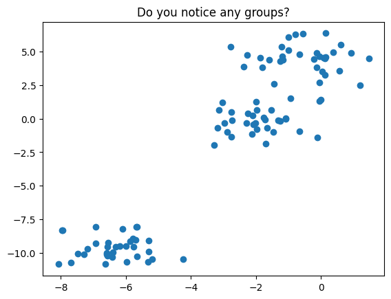
X, _ = make_blobs(random_state=11)
plt.scatter(X[:, 0], X[:, 1])
plt.title('Do you notice any groups?');
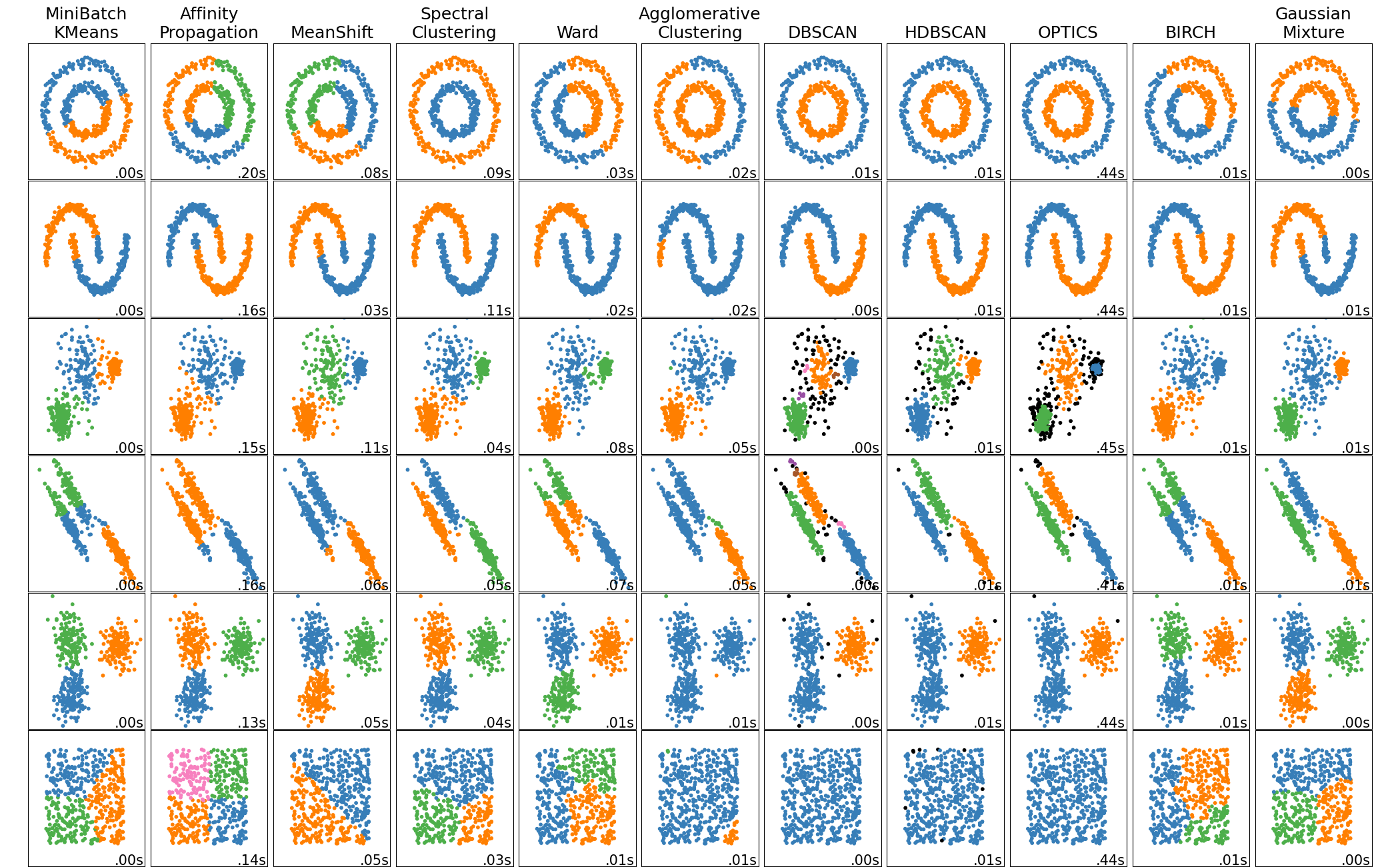
There are many clustering algorithms in sklearn – let us use the KMeans and DBSCAN approach to cluster this data.
from sklearn.cluster import KMeans, DBSCAN
from sklearn.preprocessing import StandardScaler
from sklearn.pipeline import Pipeline
Setup a pipeline to fit the KMeans clustering model, fit it to the data and plot the resulting clusters.
Evaluating Clusters#
Inertia
Sum of squared differences between each point in a cluster and that cluster’s centroid.
How dense is each cluster?
low inertia = dense cluster ranges from 0 to very high values $\( \sum_{j=0}^{n} (x_j - \mu_i)^2 \)\( where \)\mu_i$ is a cluster centroid
.inertia_ is an attribute of a fitted sklearn’s kmeans object
Silhouette Score
Tells you how much closer data points are to their own clusters than to the nearest neighbor cluster.
How far apart are the clusters?
ranges from -1 to 1 high silhouette score means the clusters are well separated $\(s_i = \frac{b_i - a_i}{max\{a_i, b_i\}}\)$ Where:
\(a_i\) = Cohesion: Mean distance of points within a cluster from each other.
\(b_i\) = Separation: Mean distance from point \(x_i\) to all points in the next nearest cluster.
Use scikit-learn: metrics.silhouette_score(X_scaled, labels).
Higher silhouette score is better!
HMMLearn#
We will use the hmmlearn library to implement our hidden markov model. Here, we use the GaussianHMM class. Depending on the nature of your data you may be interested in a different probability distribution.
HMM Learn: here
#!pip install hmmlearn
from hmmlearn import hmm
#instantiate
model = hmm.GaussianHMM(n_components=3)
#fit
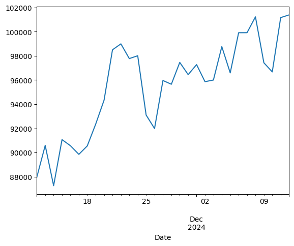
X = btcn['2021':][['Close']]
X
| Close | |
|---|---|
| Date | |
| 2024-11-12 00:00:00+00:00 | 87955.812500 |
| 2024-11-13 00:00:00+00:00 | 90584.164062 |
| 2024-11-14 00:00:00+00:00 | 87250.429688 |
| 2024-11-15 00:00:00+00:00 | 91066.007812 |
| 2024-11-16 00:00:00+00:00 | 90558.476562 |
| 2024-11-17 00:00:00+00:00 | 89845.851562 |
| 2024-11-18 00:00:00+00:00 | 90542.640625 |
| 2024-11-19 00:00:00+00:00 | 92343.789062 |
| 2024-11-20 00:00:00+00:00 | 94339.492188 |
| 2024-11-21 00:00:00+00:00 | 98504.726562 |
| 2024-11-22 00:00:00+00:00 | 98997.664062 |
| 2024-11-23 00:00:00+00:00 | 97777.281250 |
| 2024-11-24 00:00:00+00:00 | 98013.820312 |
| 2024-11-25 00:00:00+00:00 | 93102.296875 |
| 2024-11-26 00:00:00+00:00 | 91985.320312 |
| 2024-11-27 00:00:00+00:00 | 95962.531250 |
| 2024-11-28 00:00:00+00:00 | 95652.468750 |
| 2024-11-29 00:00:00+00:00 | 97461.523438 |
| 2024-11-30 00:00:00+00:00 | 96449.054688 |
| 2024-12-01 00:00:00+00:00 | 97279.789062 |
| 2024-12-02 00:00:00+00:00 | 95865.304688 |
| 2024-12-03 00:00:00+00:00 | 96002.164062 |
| 2024-12-04 00:00:00+00:00 | 98768.531250 |
| 2024-12-05 00:00:00+00:00 | 96593.570312 |
| 2024-12-06 00:00:00+00:00 | 99920.710938 |
| 2024-12-07 00:00:00+00:00 | 99923.335938 |
| 2024-12-08 00:00:00+00:00 | 101236.015625 |
| 2024-12-09 00:00:00+00:00 | 97432.718750 |
| 2024-12-10 00:00:00+00:00 | 96675.429688 |
| 2024-12-11 00:00:00+00:00 | 101173.031250 |
| 2024-12-12 00:00:00+00:00 | 101396.296875 |
model.fit(X)
GaussianHMM(n_components=3)In a Jupyter environment, please rerun this cell to show the HTML representation or trust the notebook.
On GitHub, the HTML representation is unable to render, please try loading this page with nbviewer.org.
GaussianHMM(n_components=3)
#predict
model.predict(X)
array([1, 1, 1, 1, 1, 1, 1, 1, 2, 0, 2, 0, 2, 0, 2, 0, 2, 0, 2, 0, 2, 0,
       2, 0, 2, 0, 2, 0, 2, 0, 2])
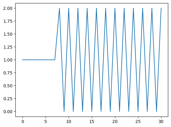
#look at our predictions
plt.plot(model.predict(X))
[<matplotlib.lines.Line2D at 0x13196e9c0>]
Looking at Speech Files#
For a deeper dive into HMM’s for speech recognition please see Rabner’s article A tutorial on hidden Markov models and selected applications in speech recognition here.
from scipy.io import wavfile
!ls sounds/apple
apple01.wav apple04.wav apple07.wav apple10.wav apple13.wav
apple02.wav apple05.wav apple08.wav apple11.wav apple14.wav
apple03.wav apple06.wav apple09.wav apple12.wav apple15.wav
#read in the data and structure
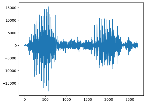
rate, apple = wavfile.read('sounds/apple/apple01.wav')
#plot the sound
plt.plot(apple)
[<matplotlib.lines.Line2D at 0x131a9e180>]
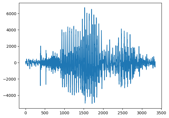
#look at another sample
rate, kiwi = wavfile.read('sounds/kiwi/kiwi01.wav')
#kiwi's perhaps
plt.plot(kiwi)
[<matplotlib.lines.Line2D at 0x131b5ab10>]
from IPython.display import Audio
#take a listen to an apple
Audio('sounds/banana/banana02.wav')
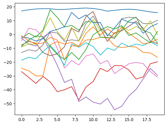
Generating Features from Audio: Mel Frequency Cepstral Coefficient#
Big idea here is to extract the important elements that allow us to identify speech. For more info on the MFCC, see here.
!pip install python_speech_features
Requirement already satisfied: python_speech_features in /Library/Frameworks/Python.framework/Versions/3.12/lib/python3.12/site-packages (0.6)
import python_speech_features as features

#extract the mfcc features
mfcc_features = features.mfcc(kiwi)

#plot them
plt.plot(mfcc_features);

#determine our x and y
X = features.mfcc(kiwi)
y = ['kiwi']
import os
#make a custom markov class to return scores
class MakeMarkov:

    def __init__(self, n_components = 3):
        self.components = n_components
        self.model = hmm.GaussianHMM(n_components=self.components)

    def fit(self, X):
        self.fit_model = self.model.fit(X)
        return self.fit_model

    def score(self, X):
        self.score = self.fit_model.score(X)
        return self.score
kiwi_model = MakeMarkov()
kiwi_model.fit(X)
kiwi_model.score(X)
-731.8623250842647
hmm_models = []
labels = []
for file in os.listdir('sounds'):
    sounds = os.listdir(f'sounds/{file}')
    sound_files = [f'sounds/{file}/{sound}' for sound in sounds]
    for sound in sound_files[:-1]:
        rate, data = wavfile.read(sound)
        X = features.mfcc(data)
        mmodel = MakeMarkov()
        mmodel.fit(X)
        hmm_models.append(mmodel)
        labels.append(file)
Model is not converging. Current: -747.3672269421642 is not greater than -747.3672268616228. Delta is -8.054132649704115e-08
Model is not converging. Current: -767.2134107023999 is not greater than -767.2134106283881. Delta is -7.401172297250014e-08
Model is not converging. Current: -737.257806389045 is not greater than -737.2578063691759. Delta is -1.9869048628606834e-08
Model is not converging. Current: -1530.590252835315 is not greater than -1530.590252515925. Delta is -3.1938998290570453e-07
#write a loop that bops over the files and prints the label based on
#highest score
Making Predictions#
Now that we have our models, given a new sound we want to score these based on what we’ve learned and select the most likely example.
in_files = ['sounds/pineapple/pineapple15.wav',
           'sounds/orange/orange15.wav',
           'sounds/apple/apple15.wav',
           'sounds/kiwi/kiwi15.wav']
Further Reading#
Textbook: Marsland’s Machine Learning: An Algorithmic Perspective has a great overview of HMM’s.
Time Series Examples: Checkout Aileen Nielsen’s tutorial from SciPy 2019 and her book Practical Time Series Analysis
Speech Recognition: Rabiner’s A tutorial on hidden Markov models and selected applications in speech recognition
HMM;s and Dynamic Programming: Avik Das’ PyData Talk Dynamic Programming for Machine Learning: Hidden Markov Models